TensorFlow2.0 Guide官方教程 学习笔记10- Eager execution

本笔记参照TensorFlow官方教程，主要是对‘Eager execution’教程内容翻译和内容结构编排，原文链接：Eager execution
目录
一、创建环境和基本使用
二、动态控制流
三、即刻训练（Eager training）
3.1计算梯度
3.2训练一个模型
3.3变量和优化器
3.4基于对象保存（objec-based saving）
3.5对象导向指标
3.6总结和TensorBoard
四、高级自动区分主体
4.1动态模型
4.2定制梯度
五、性能
基准
六、使用函数工作

---

TensorFlow的立即执行是一种命令式编程环境，它可以立即计算操作，而不需要构建图形:操作返回具体的值，而不是构建一个计算图形以供以后运行。这使得开始使用TensorFlow和调试模型变得很容易，同时也减少了样板文件。要跟随本指南，请在交互式python解释器中运行下面的代码示例。
即刻执行（Eager execution）是一个用于研究和实验的灵活的机器学习平台，提供:

• 一个直观的接口-自然地构造我们的代码并使用Python数据结构。快速迭代小模型和小数据。

• 更简单的调试-调用操作直接检查运行的模型和测试更改。使用标准的Python调试工具来立即报告错误。

• 自然控制流——使用Python控制流代替图形控制流，简化了动态模型的规范。
  即刻执行支持大多数TensorFlow操作和GPU加速。

   注意:一些模型在启用了即时执行后可能会增加开销。性能改进正在进行中，但是如果发现了问题，请提交一个bug并共享基准测试。
  

一、创建环境和基本使用

from __future__ import absolute_import, division, print_function, unicode_literals
import os

try:
  # %tensorflow_version only exists in Colab.
  %tensorflow_version 2.x  #gpu
except Exception:
  pass
import tensorflow as tf

import cProfile

在TensorFlow2.0里，即刻执行是默认使能的

tf.executing_eagerly()

True

现在我们可以运行TensorFlow操作，结果就会立即出来

x = [[2.]]
m = tf.matmul(x, x)
print("hello, {}".format(m))

hello, [[4.]]

启用立即执行将改变TensorFlow操作的行为方式，现在它们立即计算并将值返回给Python。tf.Tensor对象引用具体的值，而不是计算图中节点的符号句柄。由于在会话中没有要构建和稍后运行的计算图形，因此很容易使用print()或调试器检查结果。评估、打印和检查张量值并不会破坏梯度计算的流程。

即刻执行与Numpy结合地很好。Numpy操作接受tf.Tensor参数。TensorFlow数学操作将Python对象和Numpy数组转化为tf.TensorFlow对象。tf.Tensor.numpy方法以Numpy ndarray的形式返回对象的值。

a = tf.constant([[1, 2],
                 [3, 4]])
print(a)

tf.Tensor(
[[1 2]
 [3 4]], shape=(2, 2), dtype=int32)

# Broadcasting support
b = tf.add(a, 1)
print(b)

tf.Tensor(
[[2 3]
 [4 5]], shape=(2, 2), dtype=int32)

# Operator overloading is supported
print(a * b)

tf.Tensor(
[[ 2  6]
 [12 20]], shape=(2, 2), dtype=int32)

# Use NumPy values
import numpy as np

c = np.multiply(a, b)
print(c)

[[1 2]
 [3 4]]

二、动态控制流
立即执行的一个主要好处是，在执行模型时，宿主语言的所有功能都是可用的。例如，fizzbuzz很容易写:

def fizzbuzz(max_num):
  counter = tf.constant(0)
  max_num = tf.convert_to_tensor(max_num)
  for num in range(1, max_num.numpy()+1):
    num = tf.constant(num)
    if int(num % 3) == 0 and int(num % 5) == 0:
      print('FizzBuzz')
    elif int(num % 3) == 0:
      print('Fizz')
    elif int(num % 5) == 0:
      print('Buzz')
    else:
      print(num.numpy())
    counter += 1

fizzbuzz(15)

1
2
Fizz
4
Buzz
Fizz
7
8
Fizz
Buzz
11
Fizz
13
14
FizzBuzz

立即执行依赖于张量值得条件，并在运行时打印这些值。
三、即刻训练（Eager training）

3.1计算梯度
自动微分对于实现机器学习算法(如用于训练神经网络的反向传播)是有用的。在立即执行期间，使用tf.GradientTape来跟踪后面计算梯度的操作。
在即刻执行里我们可以用tf.GradientTape来训练并且/或者计算梯度。它对计算梯度循环特别有用。
由于在每次调用期间可能会发生不同的操作，所以所有的前向操作都会被记录到“磁带”中。要计算梯度，倒放磁带，然后弃掉。一个特定的tf.GradientTape只能计算一个梯度;后续调用抛出运行时错误。

w = tf.Variable([[1.0]])
with tf.GradientTape() as tape:
  loss = w * w

grad = tape.gradient(loss, w)
print(grad)  # => tf.Tensor([[ 2.]], shape=(1, 1), dtype=float32)

tf.Tensor([[2.]], shape=(1, 1), dtype=float32)

3.2训练一个模型
下面的示例创建一个多层模型，用于对标准MNIST手写数字进行分类。它演示了优化器和层api，以便在即刻执行环境中构建可训练的图形。

# Fetch and format the mnist data
(mnist_images, mnist_labels), _ = tf.keras.datasets.mnist.load_data()

dataset = tf.data.Dataset.from_tensor_slices(
  (tf.cast(mnist_images[...,tf.newaxis]/255, tf.float32),
   tf.cast(mnist_labels,tf.int64)))
dataset = dataset.shuffle(1000).batch(32)

# Build the model
mnist_model = tf.keras.Sequential([
  tf.keras.layers.Conv2D(16,[3,3], activation='relu',
                         input_shape=(None, None, 1)),
  tf.keras.layers.Conv2D(16,[3,3], activation='relu'),
  tf.keras.layers.GlobalAveragePooling2D(),
  tf.keras.layers.Dense(10)
])

甚至不需要训练，即刻执行可以直接调用模型并且检测输出：

for images,labels in dataset.take(1):
  print("Logits: ", mnist_model(images[0:1]).numpy())

Logits:  [[-0.0475073   0.02120854 -0.02093698  0.00966873 -0.0051422   0.00143414
   0.02826955 -0.0044364  -0.01332968  0.01066096]]

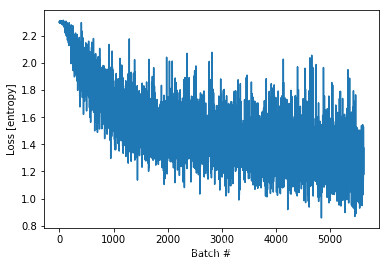
虽然keras模型有一个内置的训练循环(使用fit方法)，但有时您需要更多的定制。下面是一个用即刻执行实现的训练循环的例子:

optimizer = tf.keras.optimizers.Adam()
loss_object = tf.keras.losses.SparseCategoricalCrossentropy(from_logits=True)

loss_history = []

	注意:在tf.debug中使用assert函数来检查条件是否成立。这在即刻执行和图形执行中都有效。

def train_step(images, labels):
  with tf.GradientTape() as tape:
    logits = mnist_model(images, training=True)
    
    # Add asserts to check the shape of the output.
    tf.debugging.assert_equal(logits.shape, (32, 10))
    
    loss_value = loss_object(labels, logits)

  loss_history.append(loss_value.numpy().mean())
  grads = tape.gradient(loss_value, mnist_model.trainable_variables)
  optimizer.apply_gradients(zip(grads, mnist_model.trainable_variables))

def train():
  for epoch in range(3):
    for (batch, (images, labels)) in enumerate(dataset):
      train_step(images, labels)
    print ('Epoch {} finished'.format(epoch))

train()

Epoch 0 finished
Epoch 1 finished
Epoch 2 finished

import matplotlib.pyplot as plt

plt.plot(loss_history)
plt.xlabel('Batch #')
plt.ylabel('Loss [entropy]')

Text(0, 0.5, 'Loss [entropy]')

3.3变量和优化器
tf.Variable对象可存储tf.Tensor,就像在训练中获取的值一样，这样可以使自动区分变得更容易。
变量集合以及操作他们的方法都可以封装到层或模型中，层和模型之间的主要区别是模型添加方法的方式：Model.fit，Model.evaluate，Model.save。
举个例子，上面的自动微分的例子可以改写为：

class Linear(tf.keras.Model):
  def __init__(self):
    super(Linear, self).__init__()
    self.W = tf.Variable(5., name='weight')
    self.B = tf.Variable(10., name='bias')
  def call(self, inputs):
    return inputs * self.W + self.B

# A toy dataset of points around 3 * x + 2
NUM_EXAMPLES = 2000
training_inputs = tf.random.normal([NUM_EXAMPLES])
noise = tf.random.normal([NUM_EXAMPLES])
training_outputs = training_inputs * 3 + 2 + noise

# The loss function to be optimized
def loss(model, inputs, targets):
  error = model(inputs) - targets
  return tf.reduce_mean(tf.square(error))

def grad(model, inputs, targets):
  with tf.GradientTape() as tape:
    loss_value = loss(model, inputs, targets)
  return tape.gradient(loss_value, [model.W, model.B])

下面：
1.创建一个模型
2.代价函数对模型参数的导数
3.一种基于导数的变量更新策略。

model = Linear()
optimizer = tf.keras.optimizers.SGD(learning_rate=0.01)

print("Initial loss: {:.3f}".format(loss(model, training_inputs, training_outputs)))

for i in range(300):
  grads = grad(model, training_inputs, training_outputs)
  optimizer.apply_gradients(zip(grads, [model.W, model.B]))
  if i % 20 == 0:
    print("Loss at step {:03d}: {:.3f}".format(i, loss(model, training_inputs, training_outputs)))

Initial loss: 69.355
Loss at step 000: 66.632
Loss at step 020: 30.108
Loss at step 040: 13.900
Loss at step 060: 6.707
Loss at step 080: 3.515
Loss at step 100: 2.098
Loss at step 120: 1.469
Loss at step 140: 1.190
Loss at step 160: 1.066
Loss at step 180: 1.011
Loss at step 200: 0.987
Loss at step 220: 0.976
Loss at step 240: 0.971
Loss at step 260: 0.969
Loss at step 280: 0.968

print("Final loss: {:.3f}".format(loss(model, training_inputs, training_outputs)))

Final loss: 0.967

print("W = {}, B = {}".format(model.W.numpy(), model.B.numpy()))

W = 2.978391408920288, B = 2.0227465629577637

注意:变量持续存在，直到最后一个对python对象的引用被删除，也就是变量被删除。

3.4基于对象保存（objec-based saving）
一个tf.keras.Model包含了一个非常便捷的方法：save_weights，它让我们很容易去创建一个检查点：

model.save_weights('weights')
status = model.load_weights('weights')

使用tf.train.Checkpoint，我们可以完全控制这个过程。

x = tf.Variable(10.)
checkpoint = tf.train.Checkpoint(x=x)

x.assign(2.)   # Assign a new value to the variables and save.
checkpoint_path = './ckpt/'
checkpoint.save('./ckpt/')

'./ckpt/-1'

x.assign(11.)  # Change the variable after saving.

# Restore values from the checkpoint
checkpoint.restore(tf.train.latest_checkpoint(checkpoint_path))

print(x)  # => 2.0

<tf.Variable 'Variable:0' shape=() dtype=float32, numpy=2.0>

为了保存和加载模型，tf.train.Checkpoint存储对象的内部状态，不需要隐藏变量。要记录模型、优化器和全局步骤的状态，请将它们传递给tf.train.Checkpoint:

model = tf.keras.Sequential([
  tf.keras.layers.Conv2D(16,[3,3], activation='relu'),
  tf.keras.layers.GlobalAveragePooling2D(),
  tf.keras.layers.Dense(10)
])
optimizer = tf.keras.optimizers.Adam(learning_rate=0.001)
checkpoint_dir = 'path/to/model_dir'
if not os.path.exists(checkpoint_dir):
  os.makedirs(checkpoint_dir)
checkpoint_prefix = os.path.join(checkpoint_dir, "ckpt")
root = tf.train.Checkpoint(optimizer=optimizer,
                           model=model)

root.save(checkpoint_prefix)
root.restore(tf.train.latest_checkpoint(checkpoint_dir))

	注意：在许多训练循环中，变量是在tf.train.Checkpoint.restore被调用之后创建的。这些变量只要它们被创建就会被修复，并且可以使用断言来确保检查点已被完全加载。

3.5对象导向指标
tf.keras.metrics被存储为对象。通过将新数据传递给可调用方来更新指标，并使用tf.keras.metrics.result方法来检索结果。例如：

m = tf.keras.metrics.Mean("loss")
m(0)
m(5)
m.result()  # => 2.5
m([8, 9])
m.result()  # => 5.5

<tf.Tensor: id=669732, shape=(), dtype=float32, numpy=5.5>

3.6总结和TensorBoard
TensorBoard是一个可视化工具，用于理解、调试和优化模型训练过程。它使用在执行程序时编写的摘要事件。
我们可以使用tf.summary在即刻执行中记录变量的摘要。比如，每100个训练步骤记录一次代价摘要：

logdir = "./tb/"
writer = tf.summary.create_file_writer(logdir)

with writer.as_default():  # or call writer.set_as_default() before the loop.
  for i in range(1000):
    step = i + 1
    # Calculate loss with your real train function.
    loss = 1 - 0.001 * step
    if step % 100 == 0:
      tf.summary.scalar('loss', loss, step=step)

!ls tb/

events.out.tfevents.1571475928.c6a867357142.119.669737.v2

四、高级自动区分主体

4.1动态模型
tf.GradientTape也可以用于动态模型。这个回溯行搜索算法的例子看起来像普通的NumPy代码，除了有梯度和可微分，尽管控制流很复杂:

def line_search_step(fn, init_x, rate=1.0):
  with tf.GradientTape() as tape:
    # Variables are automatically tracked.
    # But to calculate a gradient from a tensor, you must `warch` it.
    tape.watch(init_x)
    value = fn(init_x)
  grad = tape.gradient(value, init_x)
  grad_norm = tf.reduce_sum(grad * grad)
  init_value = value
  while value > init_value - rate * grad_norm:
    x = init_x - rate * grad
    value = fn(x)
    rate /= 2.0
  return x, value

4.2定制梯度
自定义梯度是一种覆盖梯度的简单方法。在前向函数中，定义与输入、输出或中间结果相关的梯度。例如，这里有一个简单的方法剪辑的梯度规范在向后通过：

@tf.custom_gradient
def clip_gradient_by_norm(x, norm):
  y = tf.identity(x)
  def grad_fn(dresult):
    return [tf.clip_by_norm(dresult, norm), None]
  return y, grad_fn

自定义梯度广泛用于为序列操作提供数值稳定的梯度：

def log1pexp(x):
  return tf.math.log(1 + tf.exp(x))

def grad_log1pexp(x):
  with tf.GradientTape() as tape:
    tape.watch(x)
    value = log1pexp(x)
  return tape.gradient(value, x)

# The gradient computation works fine at x = 0.
grad_log1pexp(tf.constant(0.)).numpy()

0.5

# However, x = 100 fails because of numerical instability.
grad_log1pexp(tf.constant(100.)).numpy()

nan

在这里，log1pexp函数可以通过自定义梯度进行分析简化。下面的实现重用了tf.exp(x)的值，该值是在前向传递期间计算的，通过消除冗余计算使其更有效：

@tf.custom_gradient
def log1pexp(x):
  e = tf.exp(x)
  def grad(dy):
    return dy * (1 - 1 / (1 + e))
  return tf.math.log(1 + e), grad

def grad_log1pexp(x):
  with tf.GradientTape() as tape:
    tape.watch(x)
    value = log1pexp(x)
  return tape.gradient(value, x)

# As before, the gradient computation works fine at x = 0.
grad_log1pexp(tf.constant(0.)).numpy()

0.5

# And the gradient computation also works at x = 100.
grad_log1pexp(tf.constant(100.)).numpy()

1.0

五、性能

在即刻执行期间，计算会自动转移到GPU。如果我们想控制计算的运行位置，我们可以将它封装在tf.device（’/gpu:0’）块中（或等效的CPU）：

import time

def measure(x, steps):
  # TensorFlow initializes a GPU the first time it's used, exclude from timing.
  tf.matmul(x, x)
  start = time.time()
  for i in range(steps):
    x = tf.matmul(x, x)
  # tf.matmul can return before completing the matrix multiplication
  # (e.g., can return after enqueing the operation on a CUDA stream).
  # The x.numpy() call below will ensure that all enqueued operations
  # have completed (and will also copy the result to host memory,
  # so we're including a little more than just the matmul operation
  # time).
  _ = x.numpy()
  end = time.time()
  return end - start

shape = (1000, 1000)
steps = 200
print("Time to multiply a {} matrix by itself {} times:".format(shape, steps))

# Run on CPU:
with tf.device("/cpu:0"):
  print("CPU: {} secs".format(measure(tf.random.normal(shape), steps)))

# Run on GPU, if available:
if tf.config.experimental.list_physical_devices("GPU"):
  with tf.device("/gpu:0"):
    print("GPU: {} secs".format(measure(tf.random.normal(shape), steps)))
else:
  print("GPU: not found")

Time to multiply a (1000, 1000) matrix by itself 200 times:
CPU: 7.453668117523193 secs
GPU: 0.26851606369018555 secs

一个tf.Tensor对象可以复制到不同的设备来执行它的操作：

if tf.config.experimental.list_physical_devices("GPU"):
  x = tf.random.normal([10, 10])

  x_gpu0 = x.gpu()
  x_cpu = x.cpu()

  _ = tf.matmul(x_cpu, x_cpu)    # Runs on CPU
  _ = tf.matmul(x_gpu0, x_gpu0)  # Runs on GPU:0

WARNING:tensorflow:From <ipython-input-43-876293b5769c>:4: _EagerTensorBase.gpu (from tensorflow.python.framework.ops) is deprecated and will be removed in a future version.
Instructions for updating:
Use tf.identity instead.
WARNING:tensorflow:From <ipython-input-43-876293b5769c>:5: _EagerTensorBase.cpu (from tensorflow.python.framework.ops) is deprecated and will be removed in a future version.
Instructions for updating:
Use tf.identity instead.

5.1基准（Benchmarks）
对于计算量大的模型，比如在GPU上的ResNet50训练，即刻执行性能可与tf.function媲美。但是，对于计算量较少的模型，这种差距会变得更大，对于有大量小操作的模型，优化热代码路径还有很多工作要做。
六、使用函数工作
即刻执行使开发和调试更具交互性，而TensorFlow1.x风格的图形执行在分布式培训、性能优化和生产部署方面具有优势。为了弥补这一差距，TensorFlow2.0通过tf.function API引入了一些功能。详情请点击：tf.function