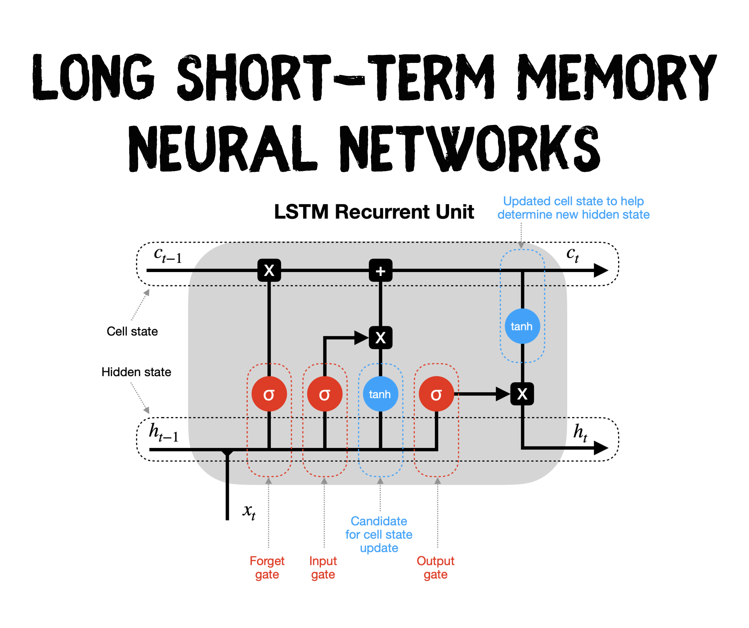
Long Short-Term Memory (LSTM) Neural Networks. Image by author.
Intro
Standard Recurrent Neural Networks (RNNs) suffer from short-term memory due to a vanishing gradient problem that emerges when working with longer data sequences.
Luckily, we have more advanced versions of RNNs that can preserve important information from earlier parts of the sequence and carry it forward. The two best-known versions are Long Short-Term Memory (LSTM) and Gated Recurrent Units (GRU).
In this article, I focus on the structure of LSTM and provide you with a detailed Python example for you to use.
Contents
Where does LSTM sit in the Machine Learning universe?
What makes LSTM different from standard RNNs and how does LSTM work?
A complete Python example showing you how to build and train your own LSTM models
Where does LSTM sit in the Machine Learning universe?
The below chart is my attempt to categorize the most common Machine Learning algorithms.
While we often use Neural Networks in a supervised manner with labelled training data, I felt that their unique approach to Machine Learning deserved a separate category.
Hence, my graph shows Neural Networks (NNs) branching out from the core of the Machine Learning universe. Recurrent Neural Networks occupy a sub-branch of NNs and contain algorithms such as standard RNNs, LSTMs, and GRUs.
The below graph is interactive, so please click on different categories to enlarge and reveal more👇 .
If you enjoy Data Science and Machine Learning, please subscribe to get an email with my new articles.
What makes LSTM different from standard RNNs and how does LSTM work?
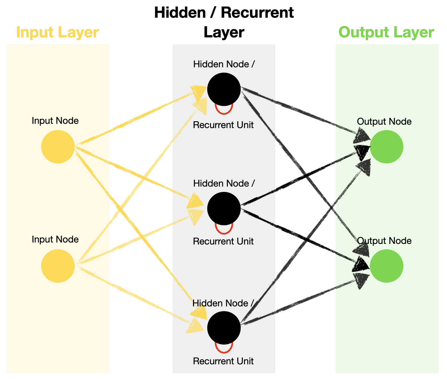
Let's start with a quick recap of a simple RNN structure. RNN consists of multiple layers similar to a Feed-Forward Neural Network: the input layer, hidden layer(s), and output layer.
Standard Recurrent Neural Network architecture. Image by author.
However, RNN contains recurrent units in its hidden layer, which allows the algorithm to process sequence data. It does it by recurrently passing a hidden state from a previous timestep and combining it with an input of the current one.
Timestep - single processing of the inputs through the recurrent unit. The number of timesteps is equal to the length of the sequence.
You can find a detailed explanation of standard RNNs in my previous article if needed.
How does LSTM differ from standard RNN?
We know that RNNs utilize recurrent units to learn from the sequence data. So do LSTMs. However, what happens inside the recurrent unit is very different between the two.
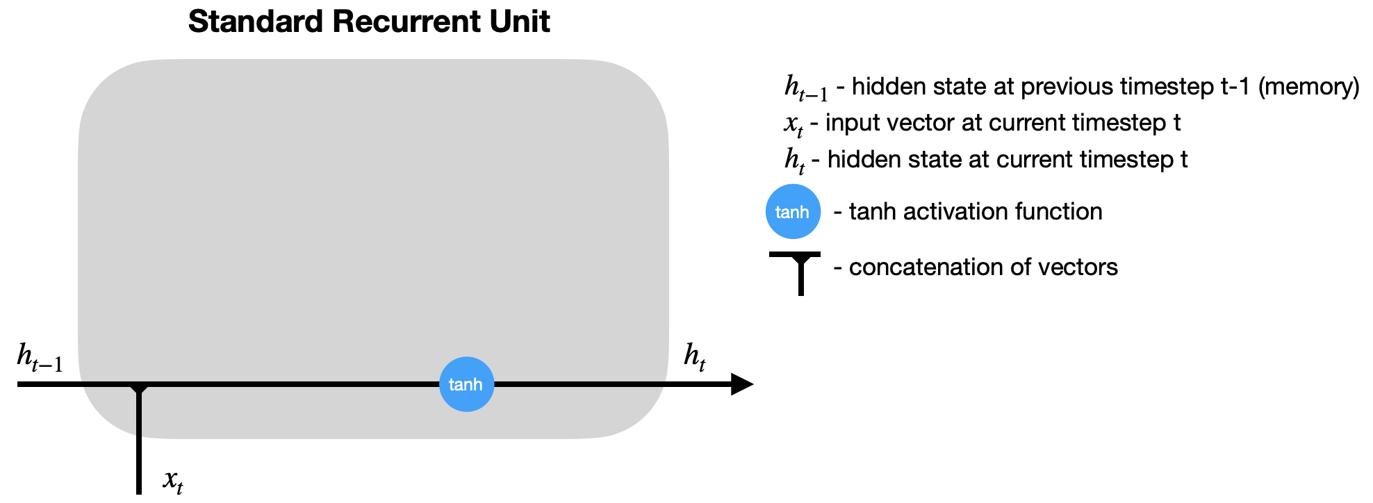
Looking inside the simplified recurrent unit diagram of a standard RNN (weights and biases not shown), we notice that there are only two major operations: combining the previous hidden state with the new input and passing it through the activation function:
After the hidden state is calculated at timestep t, it is passed back to the recurrent unit and combined with the input at timestep t+1 to calculate the new hidden state at timestep t+1. This process repeats for t+2, t+3, ..., t+n until the predefined number (n) of timesteps is reached.
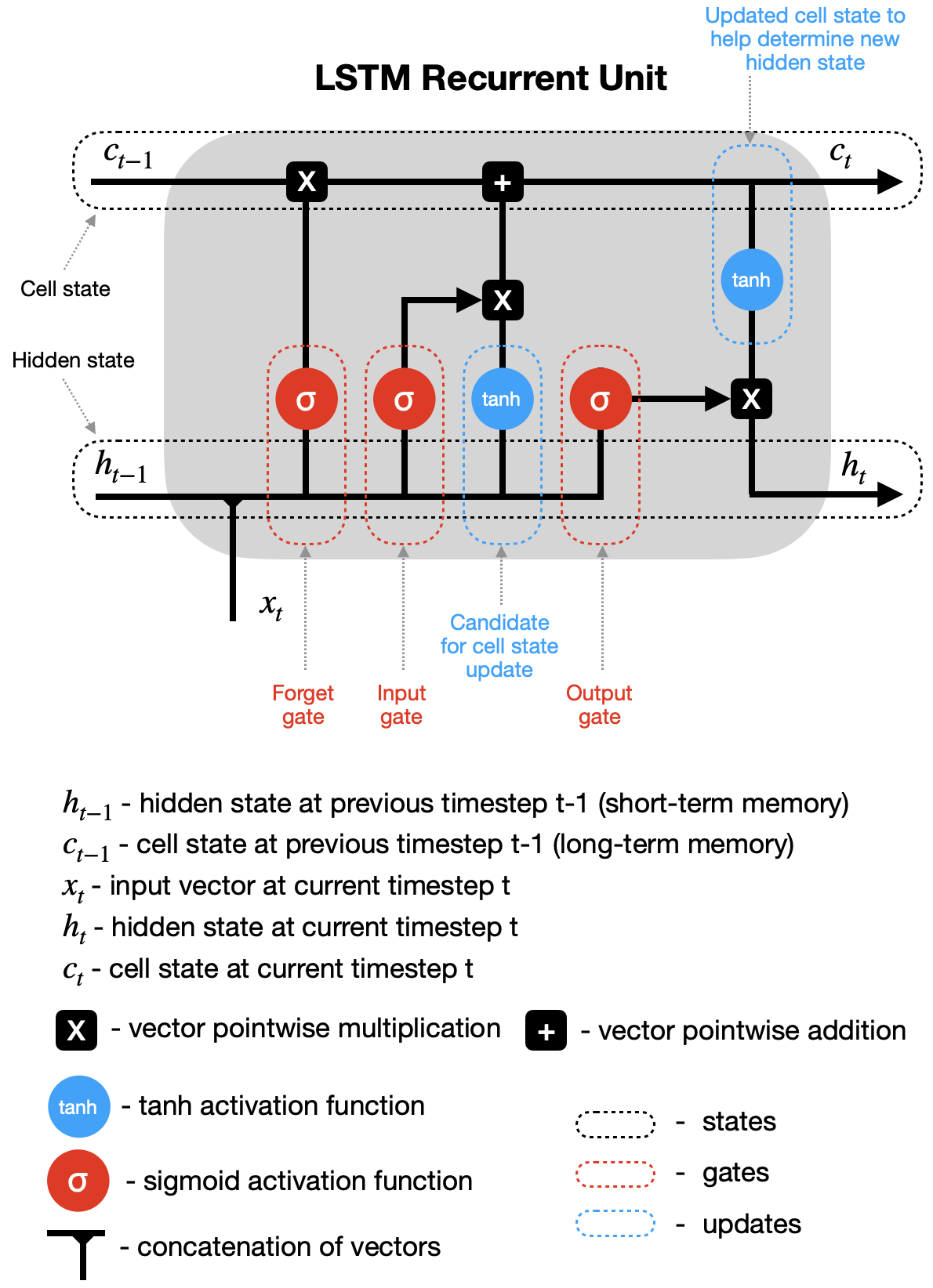
Meanwhile, LSTM employs various gates to decide what information to keep or discard. Also, it adds a cell state, which is like a long-term memory of LSTM. So let's take a closer look.
How does LSTM work?
LSTM recurrent unit is much more complex than that of RNN, which improves learning but requires more computational resources.
Let's go through the simplified diagram (weights and biases not shown) to learn how LSTM recurrent unit processes information.
Hidden state & new inputs - hidden state from a previous timestep (h_t-1) and the input at a current timestep (x_t) are combined before passing copies of it through various gates.
Forget gate - this gate controls what information should be forgotten. Since the sigmoid function ranges between 0 and 1, it sets which values in the cell state should be discarded (multiplied by 0), remembered (multiplied by 1), or partially remembered (multiplied by some value between 0 and 1).
Input gate helps to identify important elements that need to be added to the cell state. Note that the results of the input gate get multiplied by the cell state candidate, with only the information deemed important by the input gate being added to the cell state.
Update cell state -first, the previous cell state (c_t-1) gets multiplied by the results of the forget gate. Then we add new information from [input gate × cell state candidate] to get the latest cell state (c_t).
Update hidden state - the last part is to update the hidden state. The latest cell state (c_t) is passed through the tanh activation function and multiplied by the results of the output gate.
Finally, the latest cell state (c_t) and the hidden state (h_t) go back into the recurrent unit, and the process repeats at timestep t+1. The loop continues until we reach the end of the sequence.
A complete Python example showing you how to build and train your own LSTM models
We could use LSTMs in four different ways:
One-to-one - theoretically possible, but given one item is not a sequence, you don't get any benefits offered by LSTMs. Hence, it is better to use a Feed-Forward Neural Network in such a scenario instead.
Many-to-one - using a sequence of values to predict the next value. You can find a Python example of this type of setup in my RNN article.
One-to-many - using one value to predict a sequence of values.
Many-to-many - using a sequence of values to predict the next sequence of values. We will now build a many-to-many LSTM.
# Tensorflow / Kerasfrom tensorflow import keras # for building Neural Networksprint('Tensorflow/Keras: %s' % keras.__version__) # print versionfrom keras.models import Sequential # for creating a linear stack of layers for our Neural Networkfrom keras import Input # for instantiating a keras tensorfrom keras.layers import Bidirectional, LSTM, RepeatVector, Dense, TimeDistributed # for creating layers inside the Neural Network# Data manipulationimport pandas as pd # for data manipulationprint('pandas: %s' % pd.__version__) # print versionimport numpy as np # for data manipulationprint('numpy: %s' % np.__version__) # print version# Sklearnimport sklearnprint('sklearn: %s' % sklearn.__version__) # print versionfrom sklearn.preprocessing import MinMaxScaler # for feature scaling# Visualizationimport plotly import plotly.express as pximport plotly.graph_objects as goprint('plotly: %s' % plotly.__version__) # print version
The above code prints package versions I used in this example:
Next, download and ingest Australian weather data (source: Kaggle). We only ingest a subset of columns since we don't need the whole dataset for our model.
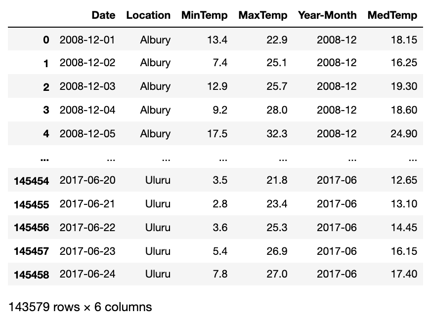
Also, we perform some simple data manipulation and derive a couple of new variables: Year-Month and Median Temperature.
python
# Set Pandas options to display more columnspd.options.display.max_columns=150# Read in the weather data csv - keep only the columns we needdf=pd.read_csv('weatherAUS.csv', encoding='utf-8', usecols=['Date', 'Location', 'MinTemp', 'MaxTemp'])# Drop records where target MinTemp=NaN or MaxTemp=NaNdf=df[pd.isnull(df['MinTemp'])==False]df=df[pd.isnull(df['MaxTemp'])==False]# Convert dates to year-monthsdf['Year-Month']= (pd.to_datetime(df['Date'], yearfirst=True)).dt.strftime('%Y-%m')# Derive median daily temperature (mid point between Daily Max and Daily Min)df['MedTemp']=df[['MinTemp', 'MaxTemp']].median(axis=1)# Show a snaphsot of datadf
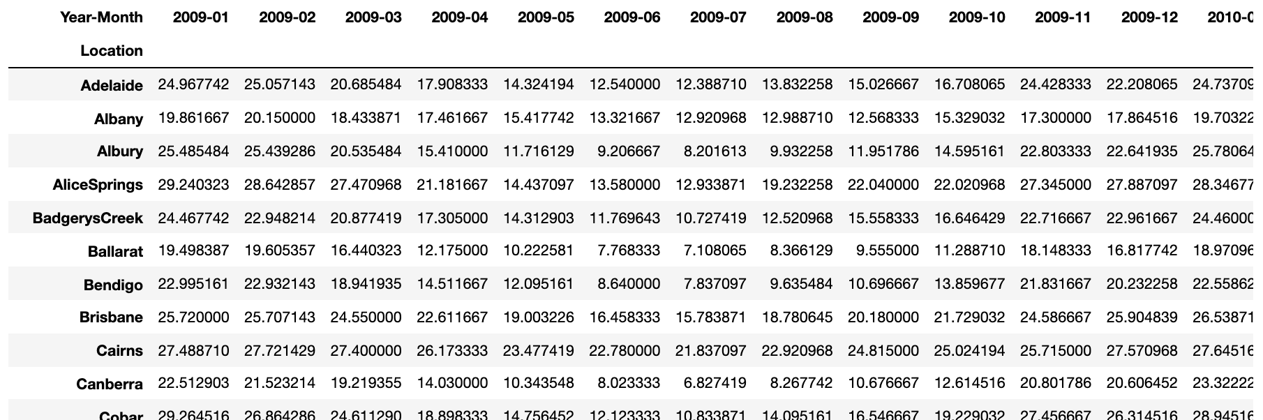
Currently, we have one Median Temperature record for each location and date. However, daily temperatures fluctuate a lot making the prediction much harder. So, let's calculate monthly averages and transpose the data to have locations as rows and Year-Months as columns.
python
# Create a copy of an original dataframedf2=df[['Location', 'Year-Month', 'MedTemp']].copy()# Calculate monthly average temperature for each locationdf2=df2.groupby(['Location', 'Year-Month'], as_index=False).mean()# Transpose dataframe df2_pivot=df2.pivot(index=['Location'], columns='Year-Month')['MedTemp']# Remove locations with lots of missing data (NaN) df2_pivot=df2_pivot.drop(['Dartmoor', 'Katherine', 'Melbourne', 'Nhil', 'Uluru'], axis=0)# Remove months with lots of missing data (NaN) df2_pivot=df2_pivot.drop(['2007-11', '2007-12', '2008-01', '2008-02', '2008-03', '2008-04', '2008-05', '2008-06', '2008-07', '2008-08', '2008-09', '2008-10', '2008-11', '2008-12', '2017-01', '2017-02', '2017-03', '2017-04', '2017-05', '2017-06'], axis=1)# Display the new dataframedf2_pivot
Average monthly temperature by location and month. Image by author.
Since we are working with real-life data, we notice that three months (2011–04, 2012–12, and 2013–02) are entirely missing from the dataframe. Therefore, we impute values for the missing months by taking an average of the preceding and subsequent month.
python
# Add missing months 2011-04, 2011-04, 2011-04 and impute datadf2_pivot['2011-04']=(df2_pivot['2011-03']+df2_pivot['2011-05'])/2df2_pivot['2012-12']=(df2_pivot['2012-11']+df2_pivot['2013-01'])/2df2_pivot['2013-02']=(df2_pivot['2013-01']+df2_pivot['2013-03'])/2# Sort columns so Year-Months are in the correct orderdf2_pivot=df2_pivot.reindex(sorted(df2_pivot.columns), axis=1)
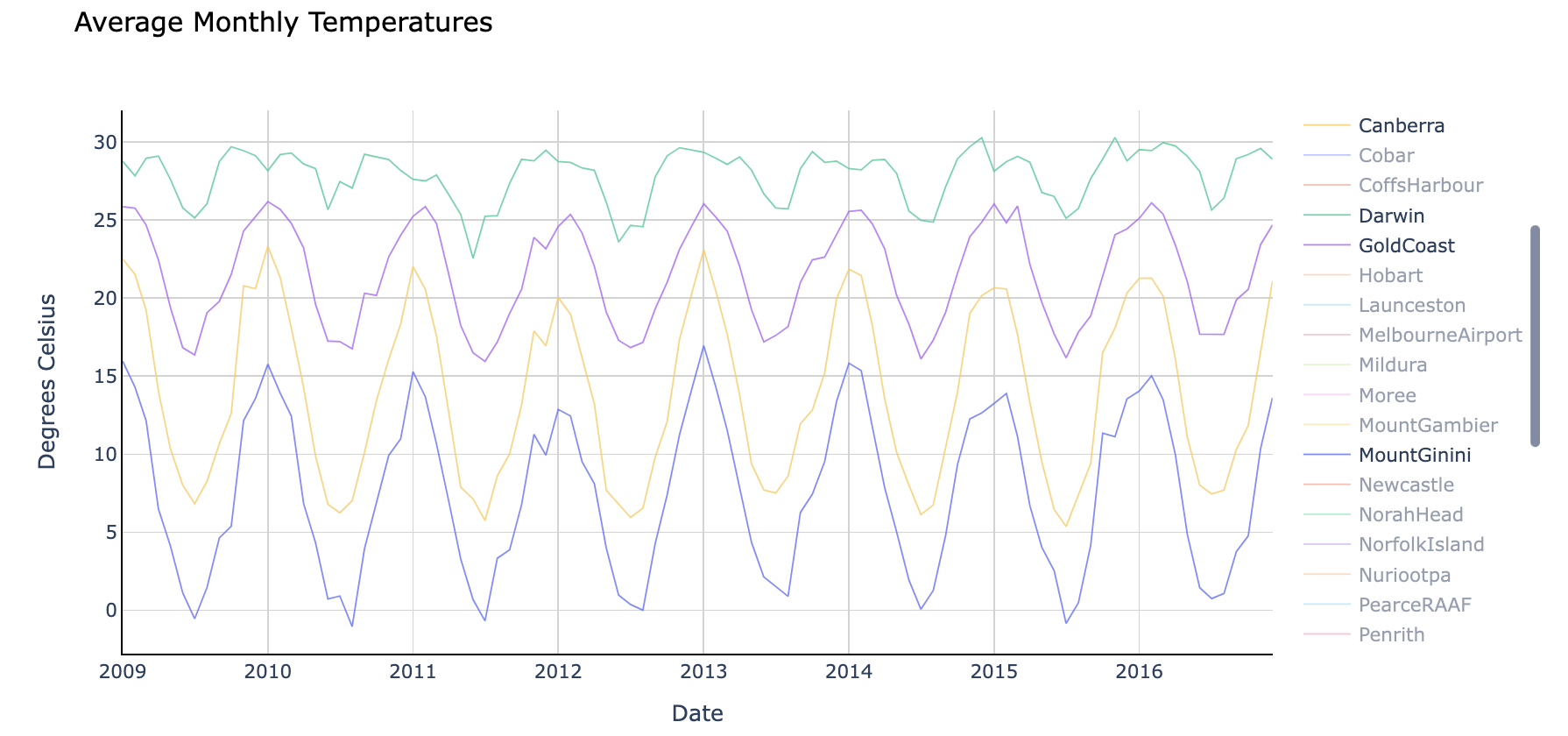
Finally, we can plot data on a chart.
python
# Plot average monthly temperature derived from daily medians for each locationfig = go.Figure()for location in df2_pivot.index: fig.add_trace(go.Scatter(x=df2_pivot.loc[location, :].index, y=df2_pivot.loc[location, :].values, mode='lines', name=location, opacity=0.8, line=dict(width=1) ))# Change chart background colorfig.update_layout(dict(plot_bgcolor = 'white'), showlegend=True)# Update axes linesfig.update_xaxes(showgrid=True, gridwidth=1, gridcolor='lightgrey', zeroline=True, zerolinewidth=1, zerolinecolor='lightgrey', showline=True, linewidth=1, linecolor='black', title='Date' )fig.update_yaxes(showgrid=True, gridwidth=1, gridcolor='lightgrey', zeroline=True, zerolinewidth=1, zerolinecolor='lightgrey', showline=True, linewidth=1, linecolor='black', title='Degrees Celsius' )# Set figure titlefig.update_layout(title=dict(text="Average Monthly Temperatures", font=dict(color='black')))fig.show()
The graph shows all locations initially, but I have picked four of them (Canberra, Darwin, Gold Coast, and Mount Ginini) to display in the above image.
Note how the mean temperature, as well as variation, differs between locations. We can either train a location-specific model for better precision, or we can train a generic model that is able to predict temperatures for every area.
In this example, I will train our LSTM model on a single location (Canberra). If you are interested in having a generic model, you can check out my follow up article on Gated Recurrent Units (GRU).
Training and evaluating LSTM model
Here are a few things to highlight before we start.
We will use sequences of 18 months to predict the average temperatures for the next 18 months. You can adjust that to your liking but beware that there will not be enough data for sequences beyond 23 months in length.
We will split the data into two separate dataframes - one for training and the other for validation (out of time validation).
Since we are creating a many-to-many prediction model, we need to use a slightly more complex encoder-decoder configuration. Both encoder and decoder are hidden LSTM layers, with information passed from one to another via a repeat vector layer.
A repeat vector is necessary when we want to have sequences of different lengths, e.g., a sequence of 18 months to predict the next 12 months. It ensures that we provide the right shape for a decoder layer. However, if your input and output sequences are of the same length as in my example, then you can also choose to set _returnsequences=True in the encoder layer and remove the repeat vector.
Note that we added a Bidirectional wrapper to LSTM layers. It allows us to train the model in both directions, which sometimes produces better results. However, its use is optional.
Also, we need to use a Time Distributed wrapper in the output layer to predict outputs for each timestep individually.
Finally, note that I have used unscaled data in this example because it has produced better results than the model trained with scaled data (MinMaxScaler). You can find both scaled and unscaled versions within Jupyter Notebooks in my GitHub repository (link available at the end of the article).
First, let's define a helper function to reshape the data to a 3D array required by LSTMs.
python
def shaping(datain, timestep): # Convert input dataframe to array and flatten arr=datain.to_numpy().flatten() cnt=0 for mth in range(0, len(datain.columns)-(2*timestep)+1): # Define range cnt=cnt+1 # Gives us the number of samples. Later used to reshape the data X_start=mth # Start month for inputs of each sample X_end=mth+timestep # End month for inputs of each sample Y_start=mth+timestep # Start month for targets of each sample. Note, start is inclusive and end is exclusive, that's why X_end and Y_start is the same number Y_end=mth+2*timestep # End month for targets of each sample. # Assemble input and target arrays containing all samples if mth==0: X_comb=arr[X_start:X_end] Y_comb=arr[Y_start:Y_end] else: X_comb=np.append(X_comb, arr[X_start:X_end]) Y_comb=np.append(Y_comb, arr[Y_start:Y_end]) # Reshape input and target arrays X_out=np.reshape(X_comb, (cnt, timestep, 1)) Y_out=np.reshape(Y_comb, (cnt, timestep, 1)) return X_out, Y_out
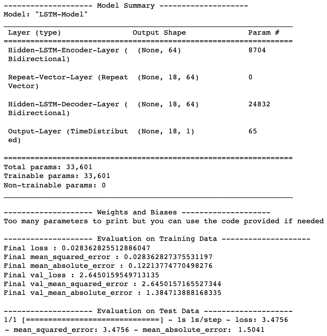
Next, we train LSTM neural network over 1,000 epochs and display a model summary with evaluation metrics. You can follow my comments within the code to understand each step.
python
##### Step 1 - Specify parameterstimestep=18location='Canberra'##### Step 2 - Prepare data# Split data into train and test dataframesdf_train=df2_pivot.iloc[:, 0:-2*timestep].copy()df_test=df2_pivot.iloc[:, -2*timestep:].copy()# Select one locationdfloc_train = df_train[df_train.index==location].copy()dfloc_test = df_test[df_test.index==location].copy()# Use previously defined shaping function to reshape the data for LSTMX_train, Y_train = shaping(datain=dfloc_train, timestep=timestep)X_test, Y_test = shaping(datain=dfloc_test, timestep=timestep)##### Step 3 - Specify the structure of a Neural Networkmodel = Sequential(name="LSTM-Model") # Modelmodel.add(Input(shape=(X_train.shape[1],X_train.shape[2]), name='Input-Layer')) # Input Layer - need to speicfy the shape of inputsmodel.add(Bidirectional(LSTM(units=32, activation='tanh', recurrent_activation='sigmoid', stateful=False), name='Hidden-LSTM-Encoder-Layer')) # Encoder Layermodel.add(RepeatVector(Y_train.shape[1], name='Repeat-Vector-Layer')) # Repeat Vectormodel.add(Bidirectional(LSTM(units=32, activation='tanh', recurrent_activation='sigmoid', stateful=False, return_sequences=True), name='Hidden-LSTM-Decoder-Layer')) # Decoder Layermodel.add(TimeDistributed(Dense(units=1, activation='linear'), name='Output-Layer')) # Output Layer, Linear(x) = x##### Step 4 - Compile the modelmodel.compile(optimizer='adam', # default='rmsprop', an algorithm to be used in backpropagation loss='mean_squared_error', # Loss function to be optimized. A string (name of loss function), or a tf.keras.losses.Loss instance. metrics=['MeanSquaredError', 'MeanAbsoluteError'], # List of metrics to be evaluated by the model during training and testing. Each of this can be a string (name of a built-in function), function or a tf.keras.metrics.Metric instance. loss_weights=None, # default=None, Optional list or dictionary specifying scalar coefficients (Python floats) to weight the loss contributions of different model outputs. weighted_metrics=None, # default=None, List of metrics to be evaluated and weighted by sample_weight or class_weight during training and testing. run_eagerly=None, # Defaults to False. If True, this Model's logic will not be wrapped in a tf.function. Recommended to leave this as None unless your Model cannot be run inside a tf.function. steps_per_execution=None # Defaults to 1. The number of batches to run during each tf.function call. Running multiple batches inside a single tf.function call can greatly improve performance on TPUs or small models with a large Python overhead. )##### Step 5 - Fit the model on the datasethistory = model.fit(X_train, # input data Y_train, # target data batch_size=1, # Number of samples per gradient update. If unspecified, batch_size will default to 32. epochs=1000, # default=1, Number of epochs to train the model. An epoch is an iteration over the entire x and y data provided verbose=0, # default='auto', ('auto', 0, 1, or 2). Verbosity mode. 0 = silent, 1 = progress bar, 2 = one line per epoch. 'auto' defaults to 1 for most cases, but 2 when used with ParameterServerStrategy. callbacks=None, # default=None, list of callbacks to apply during training. See tf.keras.callbacks validation_split=0.2, # default=0.0, Fraction of the training data to be used as validation data. The model will set apart this fraction of the training data, will not train on it, and will evaluate the loss and any model metrics on this data at the end of each epoch. #validation_data=(X_test, y_test), # default=None, Data on which to evaluate the loss and any model metrics at the end of each epoch. shuffle=True, # default=True, Boolean (whether to shuffle the training data before each epoch) or str (for 'batch'). class_weight=None, # default=None, Optional dictionary mapping class indices (integers) to a weight (float) value, used for weighting the loss function (during training only). This can be useful to tell the model to "pay more attention" to samples from an under-represented class. sample_weight=None, # default=None, Optional Numpy array of weights for the training samples, used for weighting the loss function (during training only). initial_epoch=0, # Integer, default=0, Epoch at which to start training (useful for resuming a previous training run). steps_per_epoch=None, # Integer or None, default=None, Total number of steps (batches of samples) before declaring one epoch finished and starting the next epoch. When training with input tensors such as TensorFlow data tensors, the default None is equal to the number of samples in your dataset divided by the batch size, or 1 if that cannot be determined. validation_steps=None, # Only relevant if validation_data is provided and is a tf.data dataset. Total number of steps (batches of samples) to draw before stopping when performing validation at the end of every epoch. validation_batch_size=None, # Integer or None, default=None, Number of samples per validation batch. If unspecified, will default to batch_size. validation_freq=100, # default=1, Only relevant if validation data is provided. If an integer, specifies how many training epochs to run before a new validation run is performed, e.g. validation_freq=2 runs validation every 2 epochs. max_queue_size=10, # default=10, Used for generator or keras.utils.Sequence input only. Maximum size for the generator queue. If unspecified, max_queue_size will default to 10. workers=1, # default=1, Used for generator or keras.utils.Sequence input only. Maximum number of processes to spin up when using process-based threading. If unspecified, workers will default to 1. use_multiprocessing=True, # default=False, Used for generator or keras.utils.Sequence input only. If True, use process-based threading. If unspecified, use_multiprocessing will default to False. )##### Step 6 - Use model to make predictions# Predict results on training datapred_train = model.predict(X_train)# Predict esults on test datapred_test = model.predict(X_test)##### Step 7 - Print Performance Summaryprint("")print('-------------------- Model Summary --------------------')model.summary() # print model summaryprint("")print('-------------------- Weights and Biases --------------------')print("Too many parameters to print but you can use the code provided if needed")print("")#for layer in model.layers:# print(layer.name)# for item in layer.get_weights():# print(" ", item)#print("")# Print the last value in the evaluation metrics contained within history fileprint('-------------------- Evaluation on Training Data --------------------')for item in history.history: print("Final", item, ":", history.history[item][-1])print("")# Evaluate the model on the test data using "evaluate"print('-------------------- Evaluation on Test Data --------------------')results = model.evaluate(X_test, Y_test)print("")
The above code prints the following summary and evaluation metrics for our LSTM neural network (note, your results may differ due to the stochastic nature of neural network training):
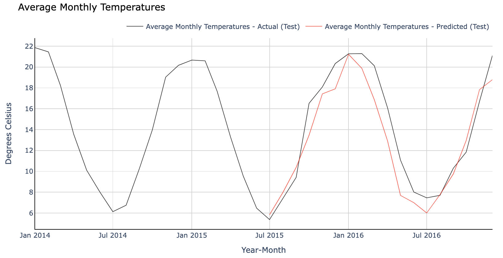
Let's now plot the results on a chart to compare actual and predicted values.
python
# Plot average monthly temperatures (actual and predicted) for test (out of time) datafig = go.Figure()# Trace for actual temperaturesfig.add_trace(go.Scatter(x=np.array(dfloc_test.columns), y=np.array(dfloc_test.values).flatten(), mode='lines', name='Average Monthly Temperatures - Actual (Test)', opacity=0.8, line=dict(color='black', width=1) ))# Trace for predicted temperaturesfig.add_trace(go.Scatter(x=np.array(dfloc_test.columns[-timestep:]), y=pred_test.flatten(), mode='lines', name='Average Monthly Temperatures - Predicted (Test)', opacity=0.8, line=dict(color='red', width=1) ))# Change chart background colorfig.update_layout(dict(plot_bgcolor = 'white'))# Update axes linesfig.update_xaxes(showgrid=True, gridwidth=1, gridcolor='lightgrey', zeroline=True, zerolinewidth=1, zerolinecolor='lightgrey', showline=True, linewidth=1, linecolor='black', title='Year-Month' )fig.update_yaxes(showgrid=True, gridwidth=1, gridcolor='lightgrey', zeroline=True, zerolinewidth=1, zerolinecolor='lightgrey', showline=True, linewidth=1, linecolor='black', title='Degrees Celsius' )# Set figure titlefig.update_layout(title=dict(text="Average Monthly Temperatures", font=dict(color='black')), legend=dict(orientation="h", yanchor="bottom", y=1.02, xanchor="right", x=1) )fig.show()
LSTM Neural Network predictions vs. actuals. Image by author.
It looks like we have been relatively successful in our quest to predict average monthly temperatures in Canberra. See if you can get better results for a different Australian city!
Final remarks
I sincerely hope you enjoyed reading this article and obtained some new knowledge.
You can find the complete Jupyter Notebook code in my GitHub repository. Feel free to use it to build your own LSTM Neural Networks, and do not hesitate to get in touch if you have any questions or suggestions.