Naive Bayes Classifier - How to Successfully Use It in Python?
A detailed explanation of the theory behind the algorithm together with 6 Python examples
Machine Learning

Preface
Just so you know what you are getting into, this is a long story that contains a mathematical explanation of the Naive Bayes classifier with 6 different Python examples. Please take a look at the list of topics below and feel free to jump to the most interesting sections for you.
Intro
Machine Learning is making huge leaps forward, with an increasing number of algorithms enabling us to solve complex real-world problems.
This story is part of a deep dive series explaining the mechanics of Machine Learning algorithms. In addition to giving you an understanding of how ML algorithms work, it also provides you with Python examples to build your own ML models.
This story covers the following topics:
Python examples of how to build Naive Bayes classification models, including:
Gaussian NB with 2 independent variables Gaussian NB with 3 class labels and 2 independent variables Categorical NB with 2 independent variables Bernoulli NB with 1 independent variable Mixed NB (Gaussian + Categorical) approach 1 - convert continuous variables into categorical ones through binning and then train a categorical model Mixed NB (Gaussian + Categorical) approach 2 - train two separate models using continuous and categorical variables and then train the final model based on predictions from the first two models
What category of algorithms does the Naive Bayes classifier belong to?
Naive Bayes classifier is based on the Bayes' Theorem, adapted for use across different machine learning problems. These include classification, clustering, and network analysis. This story will explain how Naive Bayes is used for classification problems that sit under the supervised branch of the Machine Learning tree.
Talking about supervised learning, a quick reminder of the difference between regression and classification:
Regression aims to predict the value of a continuous target variable (e.g., price of a house)
Classification aims to predict the class label of a categorical target variable (e.g., spam email / not-spam email)
The below graph is interactive, so make sure to click on different categories to enlarge and reveal more👇 .
If you enjoy Data Science and Machine Learning, please subscribe to get an email whenever I publish a new story.
How does the Naive Bayes classifier work?
Let's start by answering the following question first.
Why is Naive Bayes naive?
Naive Bayes' underlying assumption is that the predictors (attributes / independent variables) are independent of each other. This is a big assumption because it is easy to show that there is often at least some correlation between variables in real life. It is precisely this assumption of independence that makes Bayes classification "naive."
Nevertheless, the Naive Bayes algorithm has been shown time and time again to perform really well in classification problems, despite the assumption of independence. Simultaneously, it is a fast algorithm since it scales easily to include many predictors without having to handle multi-dimensional correlations.
Conditional probabilities
To understand Naive Bayes, we first need to understand conditional probabilities. For that, let's use the below example.
Assume we have a bucket filled with red and black balls. In total, there are 15 balls: 7 red and 8 black.

The probability of randomly picking a red ball out of the bucket is 7/15. You can write it as P(red) = 7/15.
If we were to draw balls one at a time without replacing them, what is the probability of getting a black ball on a second attempt after drawing a red one on the first attempt?
You can see that the above question is worded to provide us with the condition that needs to be satisfied first before the second attempt is made. That condition says that a red ball must be drawn during the first attempt.
As stated earlier, the probability of getting a red ball on the first attempt (P(red)) is 7/15. That leaves 14 balls inside a bucket with 6 red and 8 black. Hence, the probability of getting a black ball next is 8/14 = 4/7.
Bayes' theorem
The Bayes' theorem helps us calculate conditional probabilities of an event when we know the likelihood of a reverse event. Using the example above, we would write it as follows:
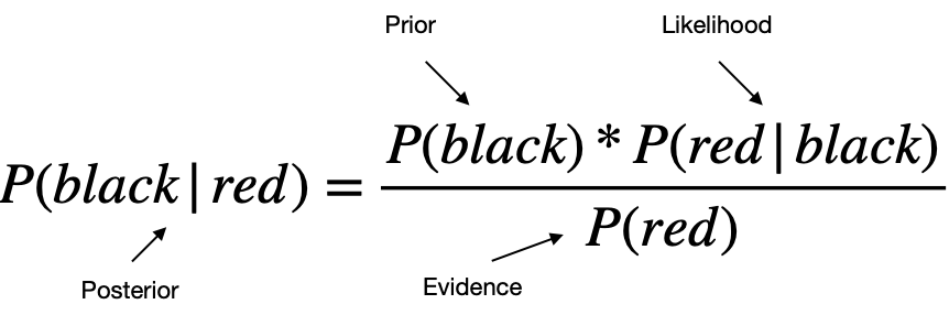
If you want to check the correctness of this, you can plug in the numbers from the above example on conditional probabilities, and you will find that both sides equal to 4/7.
Naive Bayes classifier
Let's now take the above equation and change the notation to make it more relevant for classification problems.
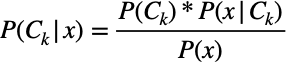
where:
P(C|x) is the posterior probability of class C (target variable) given the predictor x (attribute / independent variable);
P(C) is the prior probability of class C;
P(x|C) is the likelihood, which is the probability of the predictor x given class C;
P(x) is the prior probability of the predictor x;
Little k is just the notation to distinguish between different classes as you would have at least 2 separate classes in the classification scenario (e.g., spam / not-spam, red ball / black ball).
In practice, there is interest only in the numerator of the above equation since the denominator does not depend on C. Also, since all of the values of the attributes x are known, the denominator is effectively a constant.
So, combining the above with the assumption of independence and taking into account multiple predictors, the equation for classification becomes:

Gaussian Naive Bayes - adaptation for continuous attributes
When dealing with continuous data, a typical assumption is that each class's continuous values are distributed according to a normal (a.k.a. Gaussian) distribution.
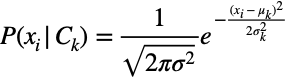
While we can use frequencies to calculate probabilities of occurrence for categorical attributes, we cannot use the same approach for continuous attributes. Instead, we first need to calculate the mean and variance for x in each class and then calculate P(x|C) using the following formula:
Bernoulli Naive Bayes - adaptation for boolean attributes
If you have binary-valued attributes (Bernoulli, boolean), then you can use a Bernoulli NB model which utilizes the following formula for calculation of P(x|C):

Note how the attribute x can only take values of 1 or 0 (true or false). Hence, the above conditional probability result is either P(i|C) or 1-P(i|C) depending on whether x is 0 or 1.
Naive Bayes usage
We have listed a lot of equations, which may seem overwhelming at this point. Don't worry, though. You can still build Naive Bayes models successfully without remembering the exact equations used in the algorithm.
The important part is identifying which Naive Bayes' variation to use given the type of attributes (independent variables) you have. This is covered in the next section.

How to build Naive Bayes models in Python?
Putting the theory behind, let's build some models in Python. We will start with Gaussian before we make our way to categorical and Bernoulli. But first, let's import data and libraries.
Setup
We will use the following:
Scikit-learn library for splitting the data into train-test samples, encoding categorical variables, building Naive Bayes models, and model evaluation
Plotly for data visualizations
Let's import all the libraries:
Then we get the chess games data from Kaggle, which you can download following this link: https://www.kaggle.com/datasnaek/chess.
Once you have saved the data on your machine, ingest it with the following code:
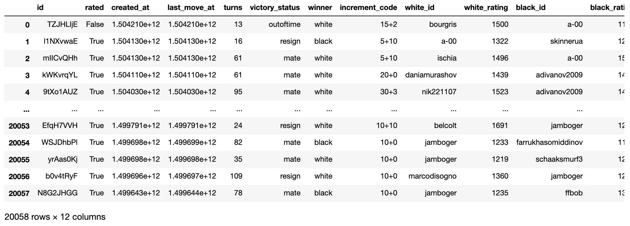
As we will want to use a 'winner' field for our dependent (target) variable, let's check the distribution of it:

We can see that wins by white and black are quite balanced. However, draws occur a lot less frequently, making it harder for the model to predict.
Nevertheless, let's prep the data by creating a few new fields for later use in the models.
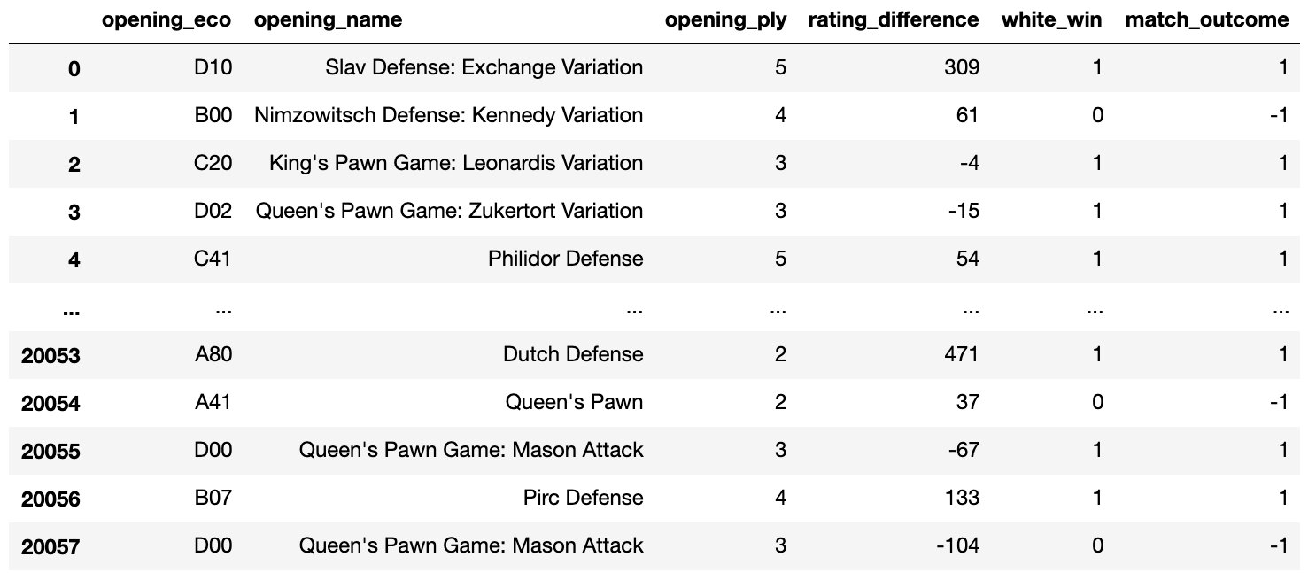
One last thing to do before we build the models is to define a function that handles sample splitting, model fitting, and printing of the results report. Calling this function will save us from repeating the same code given we will build multiple models in the below examples.
1. Gaussian NB with 2 independent variables
Let's start with a simple Gaussian Naive Bayes model. For this, we will use 'rating_difference' and 'turns' fields as our independent variables (attributes/predictors) and the 'white_win' flag as our target.
Note that we are somewhat cheating here as the number of total moves would only be known after the match. Hence, 'turns' would not be available to us if we were to make a prediction before the match starts. Nevertheless, this is for illustration purposes only, so we will go ahead and use it anyway.
After selecting the fields to use, we pass the data and algorithm name into the 'mfunc' function we defined earlier. We then get model performance results printed for our assessment.
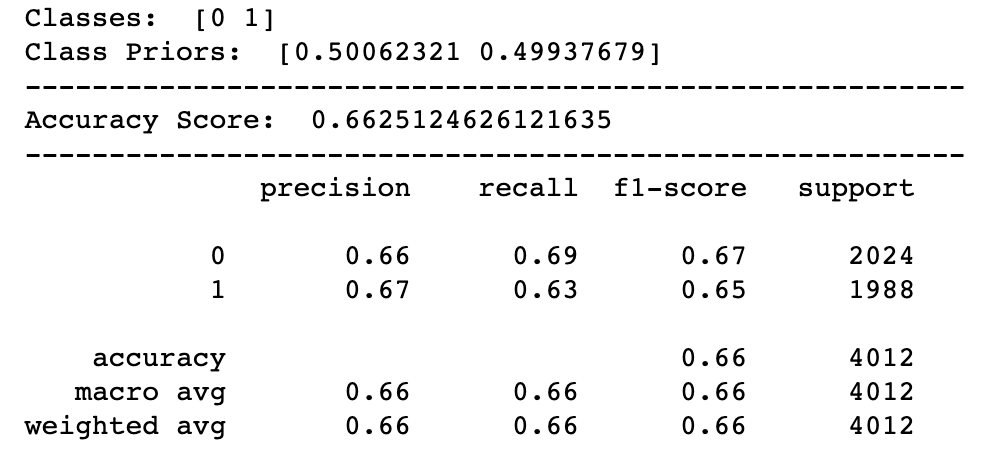
A quick recap on the performance metrics:
Accuracy = Correct predictions / Total predictions
Precision = True Positives / (True Positives + False Positives); lower precision means higher number of False Positives
Recall = True Positives / (True Positives + False Negatives); low recall means that the model contains many False Negatives, i.e., it could not correctly identify a large proportion of the class members.
F1-score = Average between Precision and Recall (weights can be applied if one metric is more important than the other for a specific use case)
Support = Number of actual observations in that class
The validation on a test sample tells us that using this model, we can correctly predict whether the white pieces win or not in 66% of the cases, which is better than a random guess (a 50% chance of getting it right). However, as stated before, we used 'turns' as one of the predictors, which in reality would not be available to us until the match was completed.
Since we only used 2 independent variables (predictors), we can easily visualize decision boundaries using the following code to create a graph.
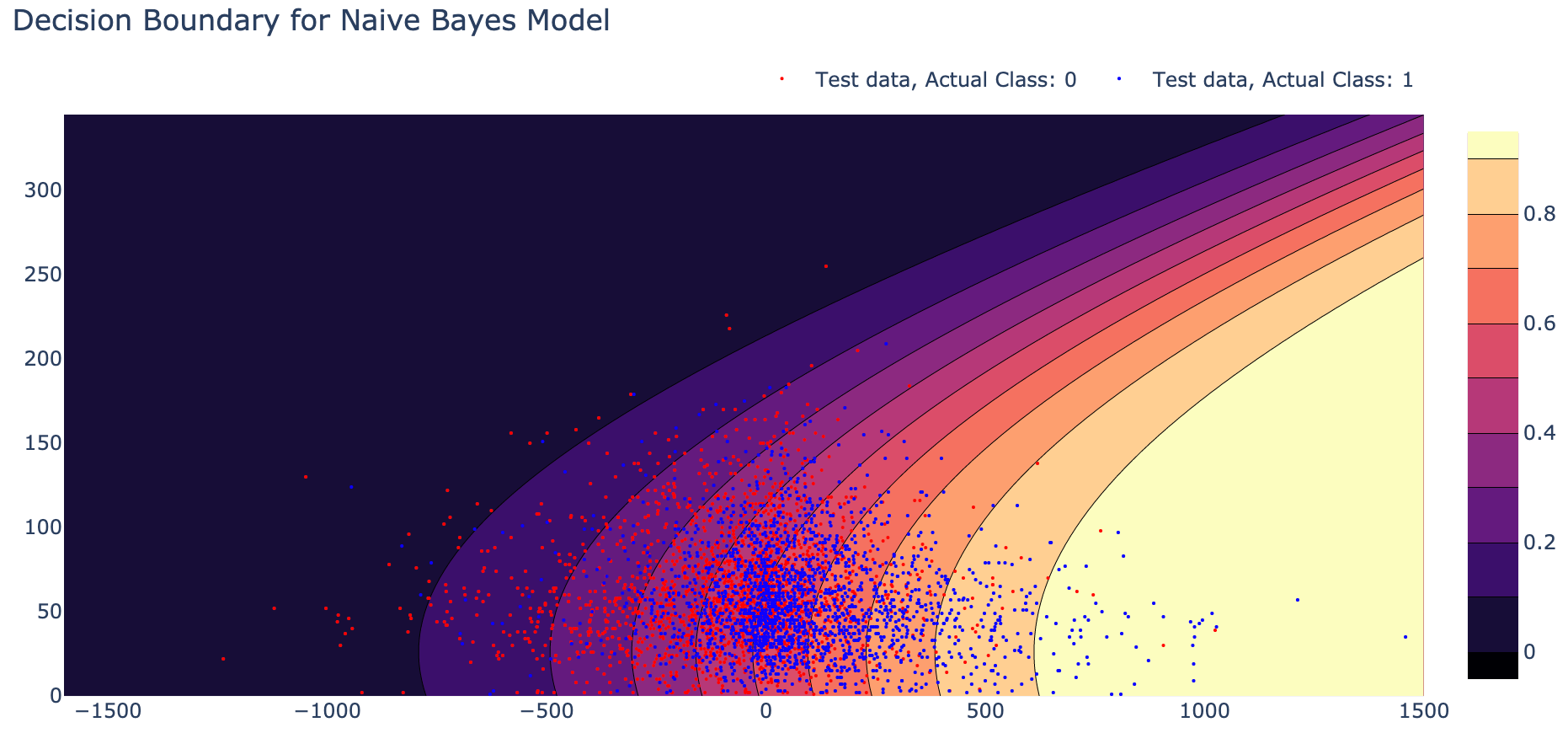
That is one nice looking graph that shows the following:
Different colors represent different probabilities of a 'white win' (class=1).
Dots are the actual outcomes, with blue being 'white win' (class=1) and red being 'white not win' (class=0).
The x-axis is the 'rating difference,' and the y-axis is the 'turns.'
As you can see, the predictions are more accurate further away from the center. This is expected, given that a significant difference in ranking represents a big difference in the skill level. Meanwhile, predictions around the decision boundary (prob=0.5) are less accurate due to the players being evenly matched and having a similar chance of winning.
2. Gaussian NB with 3 class labels and 2 independent variables
Next, let's use the same independent variables but change the target to 'match_outcome,' which has three classes:
-1: black wins
0: draw
1: white wins
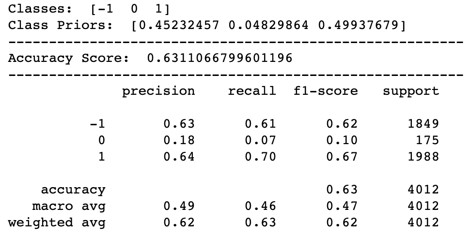
As expected, the model had some difficulty predicting class=0 (draw) due to a much smaller number of observations available for this class (only 175 in the test sample). Hence, both precision and recall metrics are very low at 0.18 and 0.07, respectively.
There are multiple ways of dealing with unbalanced data, with one approach being to oversample the minority class (in this case, class=0). I will not go into details here. However, if you are interested in oversampling, you can find a section on it in my previous story on logistic regression:
Logistic Regression in Python— A Helpful Guide to How It Works
3. Categorical NB with 2 independent variables
Next on the list is building a model using categorical independent variables. We will use 'opening_eco,' which tells us the match's opening move, and 'white_id,' which is the ID of a player playing white pieces.
Building a Categorical NB model is very similar to that of Gaussian NB but with one exception. Sklearn's package requires variables to be in a numeric format; hence we need an additional step to encode variables of a type='string' to 'numeric.' It is done with just a couple of lines using sklearn's ordinal encoder.
Quick note, the ordinal encoder is typically used to encode data that has a specific order. However, Naive Bayes' classifier in sklearn does not assume order for values of independent variables when using CategoricalNB. Hence, we are ok to use the ordinal encoder here. Otherwise, an alternative encoder would have to be used (e.g., "OneHotencoder").
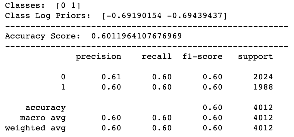
We got a model with an accuracy of 0.6, which is somewhat worse than the previous Gaussian one we built. However, we can improve on it later by combining continuous and categorical variables into one model.
4. Bernoulli NB with 1 independent variable
We want to use the Bernoulli NB model when we have binary predictor variables. For this example, we will take a field called 'rated,' which tells us whether the match was rated or not. It is a boolean field that takes values of 'True' or 'False.'
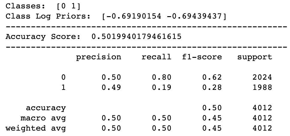
As you can see, whether the match was rated or not does not influence the match outcome. The model's accuracy and precision are both at 0.5, which means that this model is as good as a random guess.
5. Mixed NB (Gaussian + Categorical) approach 1
In this example, we will convert continuous variables into categorical ones through binning. Then we will train a categorical model on all of those features.
The code remains very similar apart from an extra step to bin continuous variables into 20% quantiles using Pandas 'qcut' method.
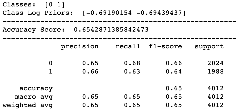
Using this approach to combine continuous and categorical variables, we managed to build the best model so far with an accuracy of 65%.
6. Mixed NB (Gaussian + Categorical) approach 2
This approach will take a bit more work as we will train two separate models using continuous and categorical independent variables. Then we will take prediction probabilities from these two models and use them for training our final model.
Since a few of the steps are different in this approach, we will not use our earlier defined 'mfunc' function. This will result in a slightly longer code.
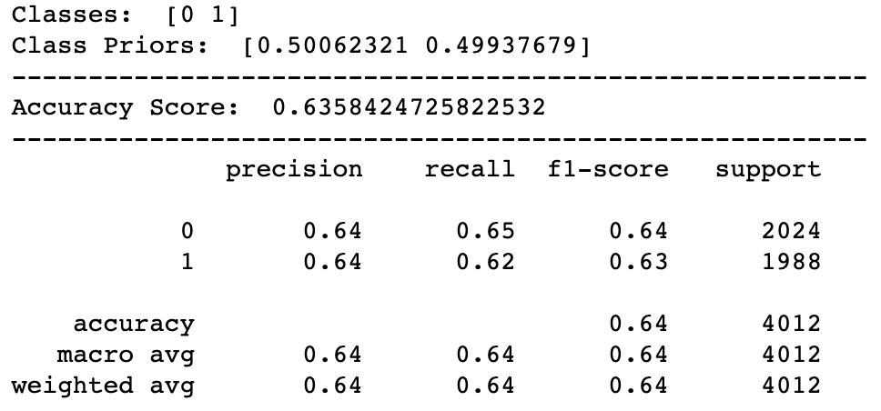
Although the model results are not as good as the previous one, this approach worked relatively well with an accuracy of 63.5%. I would suggest trying both approaches when building your model and selecting the one that works best for your data.
In conclusion
The Naive Bayes classification algorithm is very flexible and fast, and despite its 'naive' assumption, it works really well in many situations. It is definitely a good one to keep in your decision science 'toolbox.'
Feel free to use the code and other materials from this story for your own projects. I hope I managed to convey the essence of Naive Bayes. If not, please let me know how I could improve this story for other readers.
Cheers! 👏 Saul Dobilas
Related stories you may like:
BBN: Bayesian Belief Networks - How to Build Them Effectively in Python?
GMM: Gaussian Mixture Models - How to Successfully Use It to Cluster Your Data?