Swin Transformer

The Swin Transformer (Shifted Window Transformer) is a vision transformer architecture that computes self-attention within local image windows and uses a shifted window mechanism to enable interaction between neighboring regions. This allows it to efficiently learn both local and global image features.

• Learns hierarchical feature representations at multiple scales, making it effective for various computer vision tasks.
• Reduces computational cost by limiting self-attention calculations to local windows instead of the entire image.

Architecture

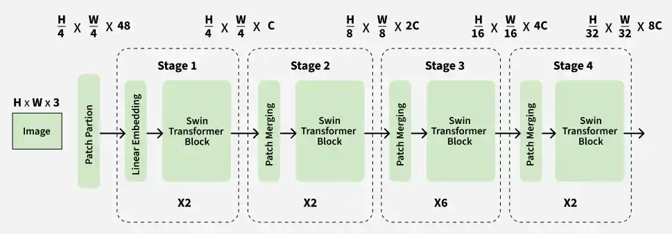
The Swin Transformer combines hierarchical feature learning with window-based self-attention to efficiently process high-resolution images.

• Patch Splitting: The input image is divided into fixed-size patches, and each patch is converted into a feature embedding.
• Window-Based Self-Attention: Self-attention is computed within local windows, allowing the model to capture local features efficiently.
• Shifted Window Attention: Window positions are shifted between layers, enabling information exchange across neighboring regions and improving global feature learning.
• Hierarchical Feature Learning: The model progressively merges patches and learns multi-scale feature representations across multiple stages.

Working

• The input image is divided into non-overlapping patches and converted into feature embeddings.
• These patches are further split into windows and self-attention is applied locally in the window.
• The windows are shifted over next layer for overlapping and self-attention is recomputed with shifted windows.
• Hierarchical processing continues combining features to know fine details in each window without losing global context of image.

Implementation

Step 1: Setup Environment

Installing the necessary libraries:

• transformers: Provides pre-trained models, including Swin Transformer.
• datasets: Loads datasets such as CIFAR-10.
• torch: Deep learning framework used to run the model.
• torchvision: Provides computer vision datasets and utilities.

!pip install transformers datasets torch torchvision

Step 2: Import Libraries

Importing the following libraries:

• Imports the Swin Transformer model and its image processor from transformers.
• load_dataset loads datasets from the Hugging Face Hub.
• torch handles tensor operations and GPU acceleration.

from transformers import AutoImageProcessor, SwinForImageClassification
from datasets import load_dataset
import torch

Step 3: Load Pre-Trained Model

Defining the Swin Transformer model name and load the pre-trained model along with its corresponding image processor for image preprocessing and classification.

model_name = "microsoft/swin-tiny-patch4-window7-224"
image_processor = AutoImageProcessor.from_pretrained(model_name)
model = SwinForImageClassification.from_pretrained(model_name)

Output:

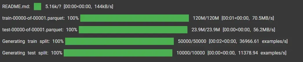
Step 4: Load Dataset

Loading the CIFAR-10 dataset, focusing on a subset for testing.

dataset = load_dataset("cifar10", split="test[:8]")

Output:

Step 5: Extract Images and Labels

Extracting the image data and corresponding ground truth labels from the dataset for classification and evaluation.

images = [item["img"] for item in dataset]
labels = [item["label"] for item in dataset]

Step 6: Preprocess Images

Preprocessing the images by resizing, normalizing, and converting them into PyTorch tensors compatible with the Swin Transformer model.

inputs = image_processor(images, return_tensors="pt").to(model.device)

Step 7: Classify Images

Setting the model to evaluation mode and perform image classification to generate prediction scores for each class.

model.eval()
with torch.no_grad():
    outputs = model(**inputs)
    logits = outputs.logits

Step 8: Process Predictions

Obtaining the predicted class labels by selecting the class with the highest score from the model's output logits.

predicted_labels = logits.argmax(dim=-1).cpu().numpy()

Step 9: Handle Label Mismatches

Handling cases where the model's output labels do not match the CIFAR-10 class labels.

• Checks whether the model's label space matches the CIFAR-10 classes.
• Maps predictions to CIFAR-10 labels when a mismatch occurs.

num_classes = len(model.config.id2label)
if num_classes != len(set(labels)):
    print("Warning: Model label space does not match CIFAR-10 labels. Mapping may be required.")
    class_mapping = {i: i % 10 for i in range(num_classes)}
    predicted_labels = [class_mapping[label] for label in predicted_labels]

Step 10: Map Predictions to Class Names

Mapping the predicted and true label indices to their human-readable class names:

class_names = [
    "airplane", "automobile", "bird", "cat", "deer", "dog", "frog", "horse", "ship", "truck"
]
predicted_class_names = [class_names[label] for label in predicted_labels]
true_class_names = [class_names[label] for label in labels]

Step 11: Print Results

Displaying the results by comparing true and predicted class names for each image:

for i, (true_label, predicted_label) in enumerate(zip(true_class_names, predicted_class_names)):
    print(
        f"Image {i + 1}: True Label = {true_label}, Predicted Label = {predicted_label}")

Output:

Image 1: True Label = cat, Predicted Label = cat
Image 2: True Label = ship, Predicted Label = ship
Image 3: True Label = ship, Predicted Label = ship
Image 4: True Label = airplane Predicted Label = bird
Image 5: True Label = frog, Predicted Label = frog
Image 6: True Label = frog, Predicted Label = ship
Image 7: True Label = automobile, Predicted Label = automobile
Image 8: True Label = frog, Predicted Label = frog

The output shows the Swin Transformer performing image classification on the CIFAR-10 dataset. Most images are classified correctly, though a few misclassifications occur because the model has not been fine-tuned on CIFAR-10.

Applications

• Image Classification: Uses a hierarchical structure and multi-scale feature extraction for highly accurate image recognition.
• Object Detection: Detects multiple objects and fine details in an image by combining local and global context.
• Image Segmentation: Segments an image into different regions using robust, multi-scale feature representations.
• Medical Imaging: Identifies anomalies and features in high-resolution medical scans, aiding diagnostics.

Advantages

• Efficient Processing: Handles high-resolution images with lower computational cost.
• Versatile: Supports tasks such as classification, detection, and segmentation.
• Reduced Complexity: More efficient than standard Vision Transformers.
• Strong Performance: Delivers accurate results across various vision applications.

Limitations

• Limited Global Context: May miss long-range dependencies in shallow networks.
• Increased Complexity: More complex to implement and tune than traditional CNNs.
• Resource Intensive: Large models require significant memory and computation.
• Weaker Local Bias: May underperform CNNs on tasks focused on highly localized features.