Create a Correlation Matrix using Python

A correlation matrix is a table that shows the relationship between multiple numerical variables in a dataset. It helps identify whether variables are positively correlated, negatively correlated, or have little to no relationship, making it useful for data analysis and feature selection.

It can be created using different Python libraries, with Pandas and NumPy being the most commonly used options.

Using NumPy Library

NumPy provides a simple way to create a correlation matrix. We can use the np.corrcoef() function to find the correlation between two or more variables.

Example: A daily sales and temperature record is kept by an ice cream store. To find the relationship between sales and temperature, we can utilize the NumPy library where x is sales in dollars and y is the daily temperature.

import numpy as np

x = [215, 325, 185, 332, 406, 522, 412, 614, 544, 421, 445, 408],
y = [14.2, 16.4, 11.9, 15.2, 18.5, 22.1, 19.4, 25.1, 23.4, 18.1, 22.6, 17.2]
res = np.corrcoef(x, y)
print(res)

[[1.         0.95750662]
 [0.95750662 1.        ]]

Using Pandas library

Pandas is used to create a correlation matrix using its built-in corr() method. It helps in analyzing and interpreting relationships between different variables in a dataset.

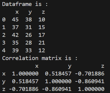
Let's create a simple DataFrame with three variables and calculate correlation matrix.

import pandas as pd

data = {'x': [45, 37, 42, 35, 39],
        'y': [38, 31, 26, 28, 33],
        'z': [10, 15, 17, 21, 12]}
        
dataframe = pd.DataFrame(data, columns=['x', 'y', 'z'])
print("Dataframe is : ")
print(dataframe)

matrix = dataframe.corr()
print("Correlation matrix is : ")
print(matrix)

Output

Using Matplotlib and Seaborn for Visualization

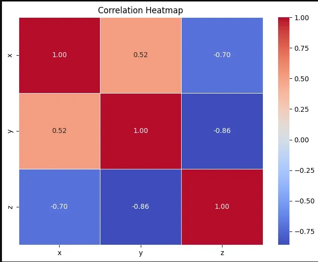
In addition to creating a correlation matrix, it is useful to visualize it. Using libraries like Matplotlib and Seaborn, we can generate heatmaps that provide a clear visual representation of how strongly variables are correlated.

import seaborn as sns
import matplotlib.pyplot as plt

matrix = dataframe.corr()
plt.figure(figsize=(8,6))
sns.heatmap(matrix, annot=True, cmap="coolwarm", fmt=".2f", linewidths=0.5)
plt.title("Correlation Heatmap")
plt.show()

Output

Example with Real Dataset (Iris Dataset)

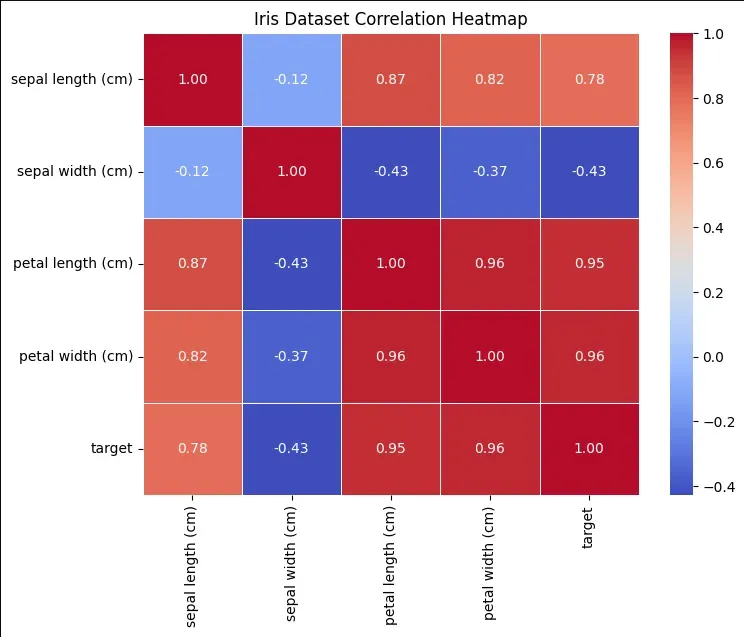
In this example we will consider Iris dataset and find correlation between the features of the dataset.

• dataset = datasets.load_iris(): Loads the Iris dataset, which includes flower feature data and species labels.
• dataframe["target"] = dataset.target: Adds a target column to the DataFrame containing the species labels.
• dataframe.corr(): Computes the correlation matrix for the numerical features in the DataFrame.
• plt.figure(figsize=(8,6)): Sets the figure size to 8 inches by 6 inches.
• sns.heatmap(matrix, annot=True, cmap="coolwarm", fmt=".2f", linewidths=0.5): Plots the correlation matrix as a heatmap, displaying values with two decimal places, using a color scale from blue (negative correlation) to red (positive correlation) and adds lines between cells for clarity.

from sklearn import datasets
import pandas as pd
import seaborn as sns
import matplotlib.pyplot as plt

dataset = datasets.load_iris()
dataframe = pd.DataFrame(data=dataset.data, columns=dataset.feature_names)
dataframe["target"] = dataset.target

matrix = dataframe.corr()

plt.figure(figsize=(8,6))
sns.heatmap(matrix, annot=True, cmap="coolwarm", fmt=".2f", linewidths=0.5)
plt.title("Iris Dataset Correlation Heatmap")
plt.show()

Output

Understanding Correlation Values

• No Correlation: A correlation value of 0 means no linear relationship between the variables. As one changes, the other does not follow any predictable pattern.
• Positive Correlation: A value closer to +1 indicates a direct relationship as one variable increases, the other also increases. Example: height and weight.
• Negative Correlation: A value closer to -1 indicates an inverse relationship as one variable increases, the other decreases. Example: speed and travel time.