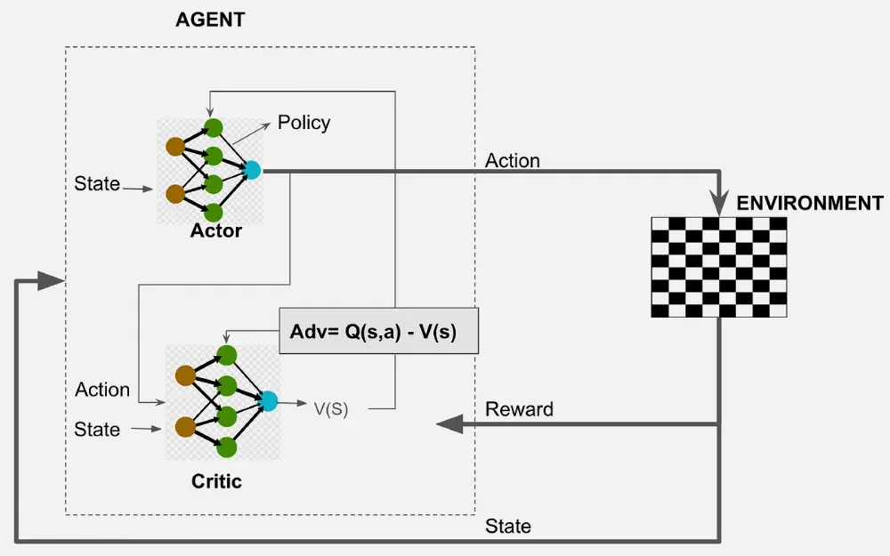
Actor-Critic Algorithm in Reinforcement Learning

Actor-Critic is a policy gradient reinforcement learning algorithm that combines two learning components: an Actor, which learns the policy for selecting actions and a Critic, which evaluates those actions by estimating the value of the current state.

By learning both the policy and value function simultaneously, the Actor-Critic algorithm achieves more stable and efficient learning than pure policy-based or value-based methods.
The Actor updates the policy to maximize long-term rewards, while the Critic provides feedback using value estimates that guide the Actor toward better decisions.

Components

1. Policy (Actor)

The policy denoted as \pi(a|s), represents the probability of taking action a in state s.
The actor seeks to maximize the expected return by optimizing this policy.
The policy is modeled by the actor network and its parameters are denoted by \theta

2. Value Function (Critic)

The value function, denoted as V(s), estimates the expected cumulative reward starting from state s.
The value function is modeled by the critic network and its parameters are denoted by w.

Working

Policy Gradient (Actor)

\nabla_\theta J(\theta)\approx \frac{1}{N} \sum_{i=0}^{N} \nabla_\theta \log\pi_\theta (a_i|s_i)\cdot A(s_i,a_i)

Here,

J(θ) represents the expected return under the policy parameterized by θ
π_\theta (a∣s) is the policy function
N is the number of sampled experiences.
A(s,a) is the advantage function representing the advantage of taking action a in state s.
i represents the index of the sample

Value Function Update (Critic)

\nabla_w J(w) \approx \frac{1}{N}\sum_{i=1}^{N} \nabla_w (V_{w}(s_i)- Q_{w}(s_i , a_i))^2

Here,

\nabla_w J(w) is the gradient of the loss function with respect to the critic's parameters w.
N is number of samples
V_w(s_i) is the critic's estimate of value of state s with parameter w
Q_w (s_i , a_i) is the critic's estimate of the action-value of taking action a
i represents the index of the sample

Update Rules

The update rules for the actor and critic involve adjusting their respective parameters using gradient ascent (for the actor) and gradient descent (for the critic).

Actor Update

\theta_{t+1}= \theta_t + \alpha \nabla_\theta J(\theta_t)

Here,

\alpha: learning rate for the actor
t is the time step within an episode

Critic Update

w_{t} = w_t -\beta \nabla_w J(w_t)

Here

w represents the parameters of the critic network
\beta is the learning rate for the critic

Advantage Function

The advantage function, A(s,a) measures the advantage of taking action a in state s over the expected value of the state under the current policy.

A(s,a)=Q(s,a)−V(s)

A positive advantage indicates that the selected action performs better than expected, whereas a negative advantage suggests that another action would likely produce a better outcome.

Training Agent: Actor-Critic Algorithm

Let's understand how the Actor-Critic algorithm works in practice. Below is an implementation of a simple Actor-Critic algorithm using TensorFlow and OpenAI Gym to train an agent in the CartPole environment.

Step 1: Import Libraries

Python

import numpy as np
import tensorflow as tf
import gymnasium as gym

Step 2: Creating CartPole Environment

Create the CartPole environment using the gym.make() function from the Gym library because it provides a standardized and convenient way to interact with various reinforcement learning tasks.

Python

# Create the CartPole Environment
env = gym.make("CartPole-v1")

Step 3: Defining Actor and Critic Networks

Actor and the Critic are implemented as neural networks using TensorFlow's Keras API.
Actor network maps the state to a probability distribution over actions.
Critic network estimates the state's value.

Python

# Define the actor and critic networks
actor = tf.keras.Sequential([
    tf.keras.layers.Input(shape=(state_dim,)),
    tf.keras.layers.Dense(32, activation="relu"),
    tf.keras.layers.Dense(action_dim, activation="softmax")
])

critic = tf.keras.Sequential([
    tf.keras.layers.Input(shape=(state_dim,)),
    tf.keras.layers.Dense(32, activation="relu"),
    tf.keras.layers.Dense(1)
])

Step 4: Defining Optimizers and Loss Functions

We use Adam optimizer for both networks.

Python

actor_optimizer = tf.keras.optimizers.Adam(learning_rate=0.001)
critic_optimizer = tf.keras.optimizers.Adam(learning_rate=0.001)

gamma = 0.99
num_episodes = 1000

Step 5: Training Loop

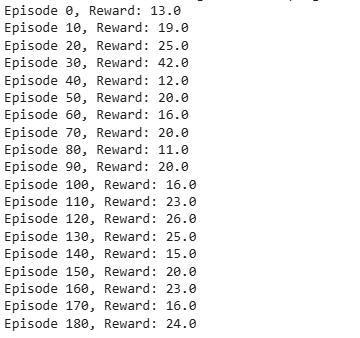
The training loop runs for 1000 episodes with the agent interacting with the environment, calculating advantages and updating both the actor and critic.

Python

for episode in range(num_episodes):

    state, _ = env.reset()
    done = False
    episode_reward = 0

    while not done:

        state_tensor = tf.convert_to_tensor([state], dtype=tf.float32)

        with tf.GradientTape() as actor_tape, tf.GradientTape() as critic_tape:

            # Actor selects action
            action_probs = actor(state_tensor)
            action = np.random.choice(action_dim, p=action_probs.numpy()[0])

            # Environment step
            next_state, reward, terminated, truncated, _ = env.step(action)
            done = terminated or truncated

            next_state_tensor = tf.convert_to_tensor([next_state], dtype=tf.float32)

            # Critic estimates values
            state_value = critic(state_tensor)[0, 0]
            next_state_value = critic(next_state_tensor)[0, 0]

            if done:
                target = reward
            else:
                target = reward + gamma * next_state_value

            advantage = target - state_value

            # Actor Loss
            actor_loss = -tf.math.log(action_probs[0, action] + 1e-8) * tf.stop_gradient(advantage)

            # Critic Loss
            critic_loss = tf.square(advantage)

        # Update Actor
        actor_grads = actor_tape.gradient(actor_loss, actor.trainable_variables)
        actor_optimizer.apply_gradients(zip(actor_grads, actor.trainable_variables))

        # Update Critic
        critic_grads = critic_tape.gradient(critic_loss, critic.trainable_variables)
        critic_optimizer.apply_gradients(zip(critic_grads, critic.trainable_variables))

        state = next_state
        episode_reward += reward

    if episode % 10 == 0:
        print(f"Episode {episode}/{num_episodes}, Reward: {episode_reward}")

# Step 7: Test the Trained Agent

state, _ = env.reset()
done = False
total_reward = 0

while not done:

    state_tensor = tf.convert_to_tensor([state], dtype=tf.float32)

    action_probs = actor(state_tensor)
    action = np.argmax(action_probs.numpy()[0])

    next_state, reward, terminated, truncated, _ = env.step(action)

    done = terminated or truncated

    total_reward += reward
    state = next_state

print("Test Total Reward:", total_reward)

env.close()

Output:

You can download the complete code from here.

Variants of Actor-Critic Algorithms

Several variants of the Actor-Critic algorithm have been developed to address specific challenges or improve performance in certain types of environments:

Advantage Actor-Critic (A2C): A2C modifies the critic’s value function to estimate the advantage function which measures how much better or worse an action is compared to the average action. The advantage function is defined as:

A(s_t, a_t) = Q(s_t, a_t) - V(s_t)

A2C helps reduce the variance of the policy gradient, leading to better learning performance.

Asynchronous Advantage Actor-Critic (A3C): A3C is an extension of A2C that uses multiple agents (threads) running in parallel to update the policy asynchronously. This allows for more stable and faster learning by reducing correlations between updates.

Applications

Robotics: Enables robots to learn navigation, manipulation and control tasks in dynamic environments.
Autonomous Vehicles: Assists self-driving cars in making safe navigation and control decisions.
Game AI: Trains intelligent agents for video games and board games with large state spaces.
Resource Management: Optimizes scheduling, resource allocation and inventory management problems.
Financial Decision-Making: Supports portfolio optimization and algorithmic trading by learning long-term strategies.

Advantages

The Critic provides value estimates that reduce the variance of policy gradient updates, resulting in more stable learning.
Learns effective policies using fewer interactions with the environment than pure policy gradient methods.
Simultaneously updating both the Actor and Critic enables quicker learning.
Can be applied to a wide variety of reinforcement learning problems.
Forms the basis of modern RL algorithms such as A2C, A3C, PPO and DDPG.

Limitations

Poor value estimates from the Critic can negatively affect the Actor's learning process.
Maintaining and training two neural networks increases computational requirements.
Performance depends heavily on selecting appropriate learning rates, discount factors and network architectures.
More difficult to implement and tune than simpler algorithms such as REINFORCE or Q-Learning.

Actor-Critic Algorithm in Reinforcement Learning

Components

1. Policy (Actor)

2. Value Function (Critic)

Working

Policy Gradient (Actor)

Value Function Update (Critic)

Update Rules

Advantage Function

Training Agent: Actor-Critic Algorithm

Step 1: Import Libraries

Step 2: Creating CartPole Environment

Step 3: Defining Actor and Critic Networks

Step 4: Defining Optimizers and Loss Functions

Step 5: Training Loop

Variants of Actor-Critic Algorithms

Applications

Advantages

Limitations

Related Articles

Explore