Random Forest for Image Classification Using OpenCV

Random Forest is a machine learning algorithm that combines multiple decision trees to improve the accuracy and stability of classification tasks. In computer vision, OpenCV is used to process and extract features from images, which can then be used as input for machine learning models like Random Forest for classification.

• OpenCV converts images into useful feature representations required for machine learning.
• Random Forest uses these features to classify images by aggregating predictions from multiple decision trees.

Step-by-Step Implementation

Used samples can be downloaded from GitHub using the link.

It can be extracted in the environment by the command:

!unzip /content/drawings.zip -d drawing

Let's see the implementation of a Random Forest to classify images using OpenCV,

Step 1: Importing the necessary libraries

• RandomForestClassifier: Trains the classification model.
• accuracy score: Measures prediction accuracy.
• os: Handles file and directory operations.
• matplotlib.pyplot: For image visualization.
• hog: Extracts HOG features.
• random: For shuffling images.
• cv2: OpenCV for image loading and preprocessing.

from sklearn.ensemble import RandomForestClassifier
from sklearn.metrics import accuracy_score
import os
import matplotlib.pyplot as plt
from skimage.feature import hog
import random
import cv2

Step 2: Define a HOG Feature Extractor

• Converts an image patch into a feature vector by analyzing gradient orientations.
• HOG helps abstract the shape and texture, robust to lighting/scale changes.

def extract_hog_features(image):
    hog_features = hog(
        image,
        orientations=9,
        pixels_per_cell=(8, 8),
        cells_per_block=(2, 2),
        visualize=False
    )
    return hog_features

Step 3: Load Images and Extract Features

• Reads each image, resizes (for uniformity & speed), converts to grayscale (reduce computation) and extracts HOG features.
• Each image is now a compact feature vector; labels are stored for classification.

def load_and_extract_features(directory):
    X, y = [], []
    for label in os.listdir(directory):
        label_dir = os.path.join(directory, label)
        for filename in os.listdir(label_dir):
            image_path = os.path.join(label_dir, filename)
            img = cv2.imread(image_path)
            img_resized = cv2.resize(img, (128, 128))
            img_gray = cv2.cvtColor(img_resized, cv2.COLOR_BGR2GRAY)
            hog_features = extract_hog_features(img_gray)
            X.append(hog_features)
            y.append(label)
    return X, y

Step 4: Train a Random Forest Classifer

• Builds an ensemble of decision trees.
• Deeper trees (higher max_depth) may overfit; 5 is a good starting point.

spiral_train_X, spiral_train_y = load_and_extract_features(
    '/content/drawings/spiral/training')
wave_train_X, wave_train_y = load_and_extract_features(
    '/content/drawings/wave/training')

spiral_rf_classifier = train_random_forest(spiral_train_X, spiral_train_y)
wave_rf_classifier = train_random_forest(wave_train_X, wave_train_y)

Step 5: Model Testing and Evaluation

• Loads and transforms test set for evaluation.
• Compares predictions vs actuals for accuracy measurement.

spiral_test_X, spiral_test_y = load_and_extract_features(
    '/content/drawings/spiral/testing')
wave_test_X, wave_test_y = load_and_extract_features(
    '/content/drawings/wave/testing')

spiral_predictions = spiral_rf_classifier.predict(spiral_test_X)
wave_predictions = wave_rf_classifier.predict(wave_test_X)

spiral_accuracy = accuracy_score(spiral_test_y, spiral_predictions)
wave_accuracy = accuracy_score(wave_test_y, wave_predictions)

print("Spiral Classification Accuracy:", spiral_accuracy)
print("Wave Classification Accuracy:", wave_accuracy)

Output:

Spiral Classification Accuracy: 0.8
Wave Classification Accuracy: 0.6333333333333333

Step 6: Visualize the Confusion Matrix

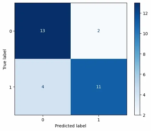
• The confusion matrix compares the actual class labels from our test data with the predicted labels from our model, providing insight into both accurate and misclassified cases for each category.
• This targeted approach ensures the confusion matrix accurately reflects model performance for the dataset currently under evaluation, allowing for focused analysis and improvement.

from sklearn.metrics import ConfusionMatrixDisplay, confusion_matrix
import matplotlib.pyplot as plt

cm = confusion_matrix(spiral_test_y, spiral_predictions)
disp = ConfusionMatrixDisplay(confusion_matrix=cm)
disp.plot(cmap=plt.cm.Blues)
plt.show()

Output:

Step 7: Visualize the Dataset and Results

def display_images(directory, num_images=5):
    fig, axes = plt.subplots(2, num_images, figsize=(15, 5))
    fig.suptitle(f"Images from {directory.split('/')[-1]}", fontsize=16)

    for i, label in enumerate(os.listdir(directory)):
        label_dir = os.path.join(directory, label)
        image_files = os.listdir(label_dir)
        random.shuffle(image_files)
        for j in range(num_images):
            image_path = os.path.join(label_dir, image_files[j])
            img = cv2.imread(image_path)
            axes[i, j].imshow(cv2.cvtColor(img, cv2.COLOR_BGR2RGB))
            axes[i, j].set_title(f"{label} Image {j+1}")
            axes[i, j].axis('off')
    plt.tight_layout()
    plt.show()

display_images('/content/drawings/spiral/training')
display_images('/content/drawings/wave/training')

display_images('/content/drawings/spiral/testing')
display_images('/content/drawings/wave/testing')

Training:

Testing:

Applications

• Medical Image Analysis and Diagnostics: Automatic detection of diseases (like Parkinson’s) from specialized image tests, e.g., analyzing spiral and wave drawings, X-rays, histopathology slides or retinal scans for early diagnosis.
• Handwriting and Digit Recognition: Classifying handwritten digits from scanned documents, forms or postal codes (e.g., MNIST dataset), useful in banking, education tech and postal services.
• Currency and Document Authentication: Detecting counterfeit notes and validating important documents by analyzing security features and visual patterns in high-resolution scans or photographs.
• Industrial Quality Control: Identifying defects, foreign objects or inconsistencies in products on assembly lines by analyzing product images for automated inspection systems.
• Facial and Biometric Identification: Recognizing individuals or verifying identity from photographs or video frames, supporting secure access or law enforcement applications.

Advantages of Using Random Forest

• Reduces Overfitting: Aggregation across many trees balances individual model quirks.
• Handles Complex Features: Well suited for high-dimensional representations from HOG or similar extractors.
• Provides Feature Importance: Offers interpretable insights about which input features drive predictions.
• Effective on Small and Medium Datasets: Especially when deep learning might be overkill or slow to train.

Disadvantages of Using Random Forest

• Resource Intensive: Large ensembles on big datasets can consume significant memory and computation time.
• Interpretability: While more transparent than neural networks, still less intuitive than single decision trees.
• Imbalanced Classes: Model performance can degrade if one class significantly outweighs another without adjustments (such as class weighting or resampling).
• Scaling to Very Large Image Sets: Not as scalable as modern deep learning architectures for millions of images or raw pixel data.