Central Limit Theorem in Statistics

The Central Limit Theorem (CLT) describes how the sample mean distribution changes with increasing sample size.

If the sample is sufficiently large (usually n > 30), then the sample means' distribution will be normally distributed regardless of the underlying population distribution, whether it is normal, skewed, or otherwise.

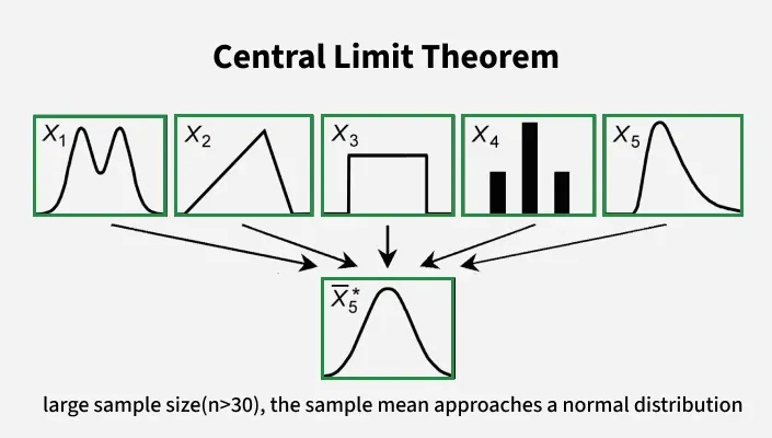
This is crucial since, even if population distribution is unknown, statisticians are able to draw inferences about the population based on the sample data. Larger samples are more accurate because CLT also proves that the distribution of the sample mean will have the mean as the population mean, and the standard deviation will reduce with increasing sample size. This theorem forms the basis for many. All types of mean distributions tend to converge to a normal distribution as the sample size increases.

The Central Limit Theorem in statistics states that as the sample size increases and its variance is finite, then the distribution of the sample mean approaches the normal distribution, irrespective of the shape of the population distribution.

Formula

Let us assume we have a random variable X. Let σ be its standard deviation, and let μ be the mean of the random variable.

• Now, as per the Central Limit Theorem, the sample mean \overline{X} will approximate a normal distribution, which is given as \overline{X} ⁓ N(μ, σ/√n).
• The Z-score of the random variable \overline{X} is given as Z =\dfrac{\overline x - \mu}{\frac{\sigma}{\sqrt n}} . Here \overline x is the mean\overline X .

The image of the formula is attached below.

Central Limit Theorem Proof

Let the independent random variables be X₁, X₂, X₃, ..., Xn, which are identically distributed and where their mean is zero (μ = 0) and their variance is one (σ² = 1).

The Z score is given as, Z = \dfrac{\overline X - \mu}{\frac{\sigma}{\sqrt n}}= \frac{\sqrt{n} (\bar{X}_n - \mu)}{\sigma}

where \bar{X}_n = \frac{1}{n} \sum_{i=1}^n X_i. \:

Here, according to the Central Limit Theorem, Z approximates to a normal distribution as the value of n increases.

i.e., Z_n \xrightarrow{d} \mathcal{N}(0,1) \quad \text{as} \quad n \to \infty

Let m(t) be the moment generating function of Xi

⇒ M(0) = 1

⇒ M'(1) = E(Xi) = μ = 0

⇒ M''(0) = E(Xi²) = 1

The Moment Generating Function for Xi/√n is given as E[e^tXi/√n]

Since X1, X₂, X₃ . . . X_n are independent, the Moment Generating Function for (X₁ + X₂ + X₃ + . . . + X_n)/√n is given as [M(t/√n)]ⁿ

Let us assume a function

f(t) = log M(t)

⇒ f(0) = log M(0) = 0

⇒ f'(0) = M'(0)/M(0) = μ/1 = μ

⇒ f''(0) = (M(0). M"(0) - M'(0)²/M'(0)² = 1

Now, using L'Hospital's Rule, we will find t/√n as t²/2

⇒ [M(t/√n)]² = [e^f(t/√n)]ⁿ

⇒ [e^nf(t/√n)] = e^(t²/2)

Thus the Central Limit Theorem has been proved by getting the Moment Generating Function of a Standard Normal Distribution.

Example: Let's say we have a large sample of observations and each sample is randomly produced and independent of other observations.

• Calculate the average of the observations, thus having a collection of averages of observations.
• Now as per the Central Limit Theorem, if the sample size is adequately large, then the probability distribution of these sample averages will approximate to a normal distribution.

Assumptions

The Central Limit Theorem is valid for the following conditions:

• The drawing of the sample from the population should be random.
• The drawing of the samples should be independent of each other.
• The sample size should not exceed ten percent of the total population when sampling is done without replacement.
• The sample size should be adequately large.
• CLT only holds for a population with finite variance.

Steps to Solve Problems

Problems of the Central Limit Theorem that involve >, <, or "between" can be solved by the following steps:

• Step 1: First identify the > and < associated with sample size, population size, mean, and variance in the problem. Also there can be 'between,; associated with a range of two numbers.
• Step 2: Draw a Graph with Mean as the Center
• Step 3: Find the Z-Score using the formula
• Step 4: Refer to the Z table to find the value of Z obtained in the previous step.
• Step 5: If the problem involves '>', subtract the Z score from 0.5; if the problem involves '<', add 0.5 to the Z score; and if the problem involves 'between,' then perform only steps 3 and 4.
• Step 6: The Z score value is found along \overline X
• Step 7: Convert the decimal value obtained in all three cases to decimal.

Mean of the Sample Mean

According to the Central Limit Theorem:

• If you have a population with a mean μ, the mean of the sample means (also called the expected value of the sample mean) will be equal to the population mean:

E(\bar{X}) = μ

Standard Deviation of the Sample Mean

The standard deviation of the sample mean (often called the standard error) describes how much the sample mean is expected to vary from the true population mean. It is calculated using the population standard deviation σ and the sample size n:

σ_Xˉ = \frac{\sigma}{\sqrt{n}}

​\sigma_{\hat{p}} = \sqrt{\frac{p(1 - p)}{n}} (For categorical data, the standard error for proportions is calculated using the true population proportion p)

Applications in Computer Science

Performance Analysis & Benchmarking

• Measuring latency/response times of systems (e.g., web servers, databases).
• The average latency over many requests converges to a normal distribution.
• Enables use of confidence intervals and parametric tests (t-tests) to compare system optimizations.

A/B Testing & Experimentation

• Comparing conversion rates between two website versions.
• User conversions are Bernoulli trials (0/1), so the average conversion rate (proportion) is approximately normal for large samples.
• Validates statistical tests (e.g., Z-tests) to determine if differences are significant. Without CLT, comparing proportions would be less straightforward.

Monte Carlo Simulations

• Estimating complex values (e.g., π, financial risks, graphics rendering) via random sampling.
• The simulation output (e.g., mean of samples) becomes normally distributed around the true value.
• Provides error bounds (e.g., "estimate ± 2 standard errors") and justifies increasing samples to reduce error.

Machine Learning (ML) & Statistics

• Used for model evaluation. Accuracy/F1-scores of ML models over test sets converge to normality, enabling comparison via confidence intervals.
• Stochastic Gradient Descent (SGD): Batch gradients are averages of random samples → approximately normal noise.
• Feature Engineering: Aggregated features (e.g., mean user interactions per day) often become Gaussian-like, simplifying assumptions for models (e.g., linear regression).

➣Practice: Solved Examples

Related Articles

• Probability Distribution Function
• Standard Deviation
• Central Tendency