
A normal distribution is a continuous probability distribution that is symmetric about its mean. In this distribution, values close to the mean occur more frequently than values farther away from the mean.
- The area under the curve of a normal distribution is always equal to 1.
- It is also known as the bell curve or Gaussian distribution.
Example: Imagine a class where students take a math test. Most students score close to the average mark, and only a few score very low or very high. If we want to describe how these marks are spread around the average in a bell-shaped pattern, this is a situation where we use the normal distribution
The formula for the probability density function of the Normal Distribution (Gaussian Distribution) is:
f(x)=\frac{1}{\sigma\sqrt{2\pi}}e^{-\frac{(x-\mu)^2}{2\sigma^2}} where:
- x = value of the random variable
- μ = mean of the distribution
- σ = standard deviation
- π ≈ 3.14159
- e ≈ 2.71828
Characteristics
- Symmetry: The normal distribution is symmetric around its mean. This means the left side of the distribution mirrors the right side.
- Mean, Median, and Mode: In a normal distribution, the mean, median, and mode are all equal and located at the center of the distribution.
- Bell-shaped Curve: The curve is bell-shaped, indicating that most of the observations cluster around the central peak and the probabilities for values further away from the mean taper off equally in both directions.
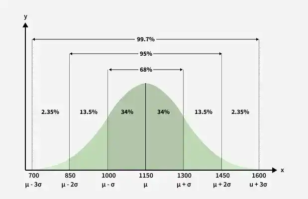
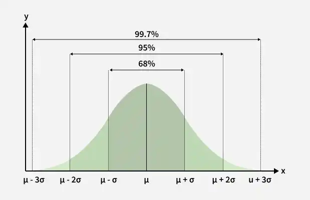
- Standard Deviation: The spread of the distribution is determined by the standard deviation. About 68% of the data falls within one standard deviation of the mean, 95% within two standard deviations, and 99.7% within three standard deviations.
- Asymptotic tails: The curve never touches the x-axis but extends infinitely.
Parameters of Normal Distribution
A normal distribution is completely determined by two parameters:
Mean (μ)
The mean represents the center of the distribution and determines the location of the peak.
- Increasing μ shifts the curve to the right.
- Decreasing μ shifts the curve to the left.
Standard Deviation (σ)
The standard deviation determines how spread out the data is around the mean.
- Smaller σ produces a narrower and taller curve.
- Larger σ produces a wider and flatter curve.
Empirical Rule of Standard Deviation
Generally, the normal distribution has a positive standard deviation, and the standard deviation divides the area of the normal curve into smaller parts, and each part defines the percentage of data that falls into a specific region. This is called the Empirical Rule of Standard Deviation in Normal Distribution.
Empirical Rule states that,
- Approximately 68% of data lies within 1 standard deviation of the mean.
- Approximately 95% of data lies within 2 standard deviations of the mean.
- Approximately 99.7% of data lies within 3 standard deviations of the mean.
This rule is known as the Empirical Rule or 68–95–99.7 Rule.
Normal Distribution Table
Normal Distribution Table, which is also called Normal Distribution Z Table, is the table of z-values for normal distribution. This Normal Distribution Z Table is given as follows:
| Z-Value | 0 | 0.01 | 0.02 | 0.03 | 0.04 | 0.05 | 0.06 | 0.07 | 0.08 | 0.09 |
|---|---|---|---|---|---|---|---|---|---|---|
| 0 | 0 | 0.004 | 0.008 | 0.012 | 0.016 | 0.0199 | 0.0239 | 0.0279 | 0.0319 | 0.0359 |
| 0.1 | 0.0398 | 0.0438 | 0.0478 | 0.0517 | 0.0557 | 0.0596 | 0.0636 | 0.0675 | 0.0714 | 0.0753 |
| 0.2 | 0.0793 | 0.0832 | 0.0871 | 0.091 | 0.0948 | 0.0987 | 0.1026 | 0.1064 | 0.1103 | 0.1141 |
| 0.3 | 0.1179 | 0.1217 | 0.1255 | 0.1293 | 0.1331 | 0.1368 | 0.1406 | 0.1443 | 0.148 | 0.1517 |
| 0.4 | 0.1554 | 0.1591 | 0.1628 | 0.1664 | 0.17 | 0.1736 | 0.1772 | 0.1808 | 0.1844 | 0.1879 |
| 0.5 | 0.1915 | 0.195 | 0.1985 | 0.2019 | 0.2054 | 0.2088 | 0.2123 | 0.2157 | 0.219 | 0.2224 |
| 0.6 | 0.2257 | 0.2291 | 0.2324 | 0.2357 | 0.2389 | 0.2422 | 0.2454 | 0.2486 | 0.2517 | 0.2549 |
| 0.7 | 0.258 | 0.2611 | 0.2642 | 0.2673 | 0.2704 | 0.2734 | 0.2764 | 0.2794 | 0.2823 | 0.2852 |
| 0.8 | 0.2881 | 0.291 | 0.2939 | 0.2967 | 0.2995 | 0.3023 | 0.3051 | 0.3078 | 0.3106 | 0.3133 |
| 0.9 | 0.3159 | 0.3186 | 0.3212 | 0.3238 | 0.3264 | 0.3289 | 0.3315 | 0.334 | 0.3365 | 0.3389 |
| 1 | 0.3413 | 0.3438 | 0.3461 | 0.3485 | 0.3508 | 0.3531 | 0.3554 | 0.3577 | 0.3599 | 0.3621 |
Applications
- Feature Scaling in Machine Learning: Data is standardized using Z-score normalization to improve model performance.
- Bayesian Inference: Gaussian distributions are widely used as prior distributions in Bayesian models.
- Anomaly Detection: Values that lie far from the mean are treated as anomalies or outliers.
- Gaussian Mixture Models: Used in clustering and unsupervised learning.
- Image Processing: Gaussian blur applies a normal-distributed kernel to reduce image noise.
- Generative AI: Diffusion models use Gaussian noise during image generation.
➣Practice: Solved Examples
