

Geospatial data represents information associated with geographic locations such as countries, cities, roads, buildings, and natural features. In Python, geospatial data can be analyzed, transformed, and visualized using libraries such as GeoPandas and GeoPlot. These libraries make it easy to work with shapefiles, perform spatial operations, and create geographic visualizations.
Libraries Used
- GeoPandas: Used for reading, analyzing, and visualizing geospatial data in Python.
- GeoPlot: Used for creating maps and geospatial visualizations from GeoPandas data.
Installation
Install GeoPandas and GeoPlot using either pip or conda.
Using pip
pip install geopandas geoplot
Using conda
conda install -c conda-forge geopandas geoplot
Note: conda-forge channel is recommended because it provides GeoPandas and its geospatial dependencies in a pre-configured environment.
After installation, you can start working with geospatial datasets immediately. Here, we use the Natural Earth Countries Dataset, which is loaded directly from its URL using GeoPandas, so no manual download is required.
Note: If you want to download the dataset locally, you can click here.
Reading a Shapefile
GeoPandas provides the read_file() function to load geospatial datasets such as Shapefiles, GeoJSON files and GeoPackages into a GeoDataFrame.
Syntax:
geopandas.read_file(filepath)
Example: Loading the Natural Earth countries shapefile into a GeoDataFrame.
import geopandas as gpd
world_data = gpd.read_file("https://naturalearth.s3.amazonaws.com/110m_cultural/ne_110m_admin_0_countries.zip")
world_data.head()
Output:
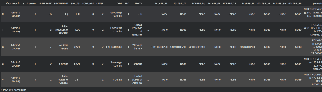
Explanation:
- gpd.read_file() reads the shapefile and loads it as a GeoDataFrame.
- world_data stores both attribute data and geometry information.
- head() displays the first five records of the dataset for inspection.
Note: GeoPandas can read spatial data directly from a local file or a URL. In Google Colab, you can load the Natural Earth dataset directly from its URL without manually downloading or uploading the shapefile files.
Plotting Geospatial Data
Once the dataset is loaded into a GeoDataFrame, you can visualize it using plot() method. GeoPandas provides a built-in plotting interface that makes it easy to create maps directly from geographic data.
Syntax:
GeoDataFrame.plot()
Example: In this example, we plot the world dataset loaded from a GeoJSON file.
url = "https://raw.githubusercontent.com/nvkelso/natural-earth-vector/master/geojson/ne_110m_admin_0_countries.geojson"
world_data = gpd.read_file(url)
world_data.plot()
Output:
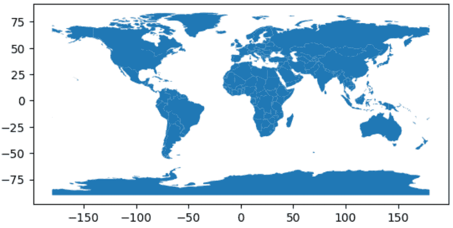
Explanation:
- gpd.read_file() loads the geographic dataset into a GeoDataFrame.
- plot() draws the geometries stored in the geometry column.
- Each country polygon is rendered automatically on the map.
- GeoPandas uses Matplotlib internally to generate the visualization.
Verifying Data Type
You can verify the data type by running:
type(world_data)
Output:

Selecting Columns
A GeoDataFrame can contain multiple attribute columns along with a geometry column. If you only need specific information, you can select the required columns just like a Pandas DataFrame.
Syntax:
data[['column1', 'column2']]
Example: In this example, we select only the country name and geometry columns from the dataset.
world_data = world_data[['NAME', 'geometry']]
world_data.head()
Output:
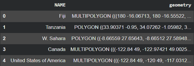
Explanation:
- [['NAME', 'geometry']] selects only the specified columns from the GeoDataFrame.
- NAME contains the country names and geometry stores the geographic boundaries of each country.
- Selecting only the required columns helps simplify the dataset and makes further analysis easier.
Computing Area of Countries
Geopandas allows to compute the area of geographic features using the .area property. Before calculating area, the data should be converted to a projected coordinate reference system to ensure accurate results.
Syntax:
GeoSeries.area
Example: In this example, we calculate the area of each country using GeoPandas. We then store the result in a new column called area.
world_data = world_data[['NAME', 'geometry']].copy()
world_data = world_data.to_crs(epsg=3857)
world_data['area'] = world_data.area
world_data.head()
Output:
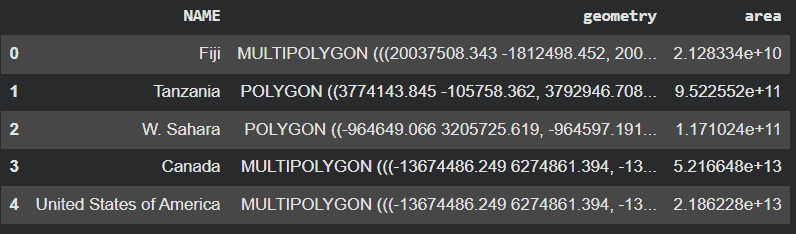
Explanation:
- [['NAME', 'geometry']].copy() prevents Pandas warning by creating a safe copy.
- to_crs(epsg=3857) converts data to a projected CRS (Web Mercator) for correct area computation.
- .area calculates the actual geometric area in square meters and result is stored in a new column area.
Filtering Countries
Filtering allows us to select or remove specific rows from a dataset based on column values. It is commonly used when we want to focus on a subset of data, such as excluding unwanted regions like Antarctica before visualization or analysis.
Syntax:
data[data['attribute'] != 'element']
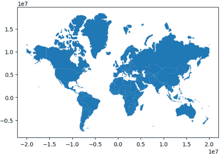
Example: In this example, we remove the continent Antarctica before plotting the map.
world_data = world_data[world_data['NAME'] != 'Antarctica']
world_data.plot()
Output:
Explanation:
- world_data['NAME'] != 'Antarctica' filters out Antarctica rows
- .plot() visualizes the filtered world map
Plotting a Specific Country
To visualize only a particular country instead of displaying the entire world map can be done by filtering the GeoDataFrame based on a country name and then plotting the resulting geometry.
Syntax:
data[data.attribute == "element"].plot()
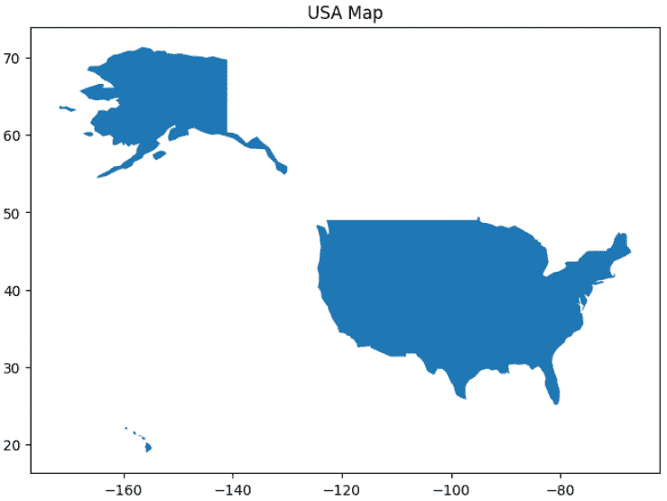
Example: In this example, we filter the dataset to select United States of America from the NAME column and display its geographic boundary.
world_data[world_data.NAME == "United States of America"].plot()
Output:
Explanation:
- world_data.NAME == "United States of America" creates a condition that selects only rows where the country name is United States of America.
- world_data[...] filters the GeoDataFrame using this condition.
Note: The maps shown in this article are generated using publicly available sample datasets provided by GeoPandas/GeoPlot. Administrative and international boundaries displayed in these datasets may vary depending on the data source and version used
Coordinate Reference System (CRS)
A Coordinate Reference System (CRS) defines how geographic coordinates (latitude and longitude) are represented on a map. It is essential for accurate spatial analysis, especially when performing operations like area calculation or map projections.
We can check the current CRS of a GeoDataFrame and also transform it into another projection using EPSG codes.
Syntax:
GeoDataFrame.crs
GeoDataFrame.to_crs(crs=None, epsg=None, inplace=False)
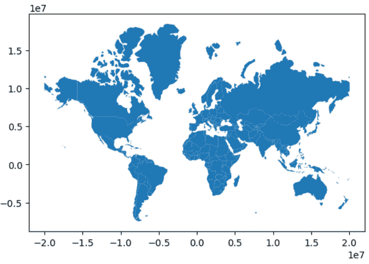
Example: In this example, we check the current CRS, convert the dataset to a projected CRS (EPSG:3857) and then visualize the map.
current_crs = world_data.crs
world_data = world_data.to_crs(epsg=3857)
world_data.plot()
Output:
Explanation:
- world_data.crs checks the current coordinate reference system.
- to_crs(epsg=3857) converts the data into a projected CRS for better spatial accuracy.
Color Mapping
Color mapping helps visualize geospatial data by assigning different colors to different regions based on a column value. This makes it easier to distinguish countries or features on a map at a glance. GeoPandas supports various colormaps from Matplotlib to enhance map readability and visualization.
Syntax:
GeoDataFrame.plot(column='attribute', cmap='colormap_name')
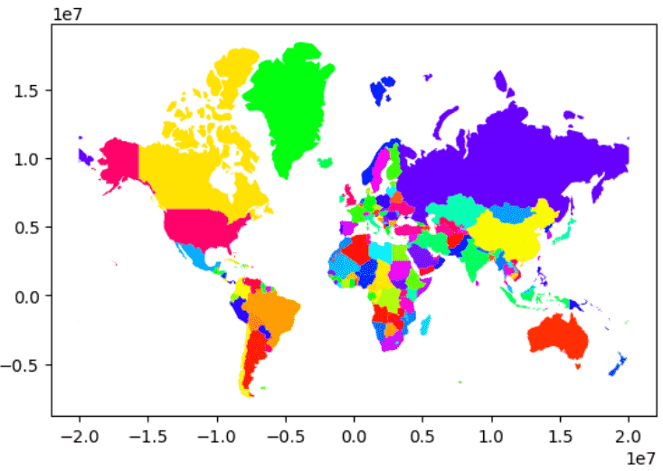
Example: In this example, we color each country based on its NAME column using the hsv colormap. We also prepare the dataset by selecting required columns and handling geometry properly.
world_data = world_data.to_crs(epsg=3857)
world_data.plot(column='NAME', cmap='hsv')
Output:
Explanation:
- to_crs(epsg=3857) converts data into a projected coordinate system for proper plotting.
- plot(column='NAME', cmap='hsv') assigns different colors to countries based on their name using the HSV colormap.
Adding a Legend
A legend helps interpret the meaning of colors in a geospatial plot, especially when data values (like area) are visualized. In GeoPandas, we can easily add legends using the legend parameter along with customization options through legend_kwds.
Syntax:
GeoDataFrame.plot(column='attribute', legend=True, legend_kwds={...})
Example: In this example, we calculate the area of each country, convert it into square kilometers, and then visualize it with a color-based legend representing country area.
world_data['area'] = world_data.area / 1_000_000
world_data.plot(
    column='area',
    cmap='hsv',
    legend=True,
    legend_kwds={'label': "Area of the country (Sq. Km.)"},
    figsize=(7, 7)
)
Output:
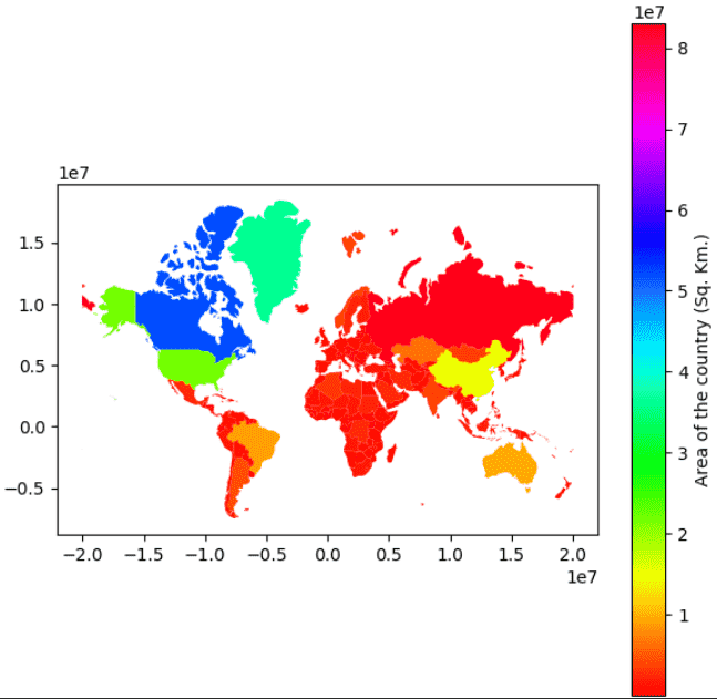
Explanation:
- area / 1_000_000 converts square meters to square kilometers.
- plot(column='area') colors countries based on their area values.
- legend=True adds a color legend to interpret values.
- legend_kwds customizes the legend label for clarity.
Resizing Legends
When working with geospatial visualizations, legends can sometimes appear too small or misaligned. GeoPandas allows better control over legend placement and size using Matplotlib’s Axes system along with make_axes_locatable.
Example: In this example, we plot country areas and customize the legend size by creating a separate axis for the colorbar using axes_grid1.
import matplotlib.pyplot as plt
from mpl_toolkits.axes_grid1 import make_axes_locatable

fig, ax = plt.subplots(figsize=(10, 10))
divider = make_axes_locatable(ax)
cax = divider.append_axes("right", size="7%", pad=0.1)

world_data.plot(
    column='area',
    cmap='hsv',
    legend=True,
    legend_kwds={'label': "Area of the country (Sq. Km.)"},
    ax=ax,
    cax=cax
)
Output:
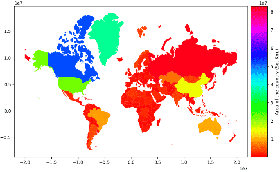
Explanation:
- fig, ax = plt.subplots() creates the main plotting area.
- make_axes_locatable(ax) allows custom layout control.
- append_axes() creates a separate axis for the legend.
- ax=ax, cax=cax ensures plot and legend are linked properly.
Polyplot and Pointplot
GeoPandas allows us to visualize geospatial data using simple plotting methods. We can plot polygon data (countries, regions) and point data (cities, locations) directly without needing extra complexity. This makes it easy to explore different spatial datasets using built-in visualization support.
Syntax:
GeoDataFrame.plot()
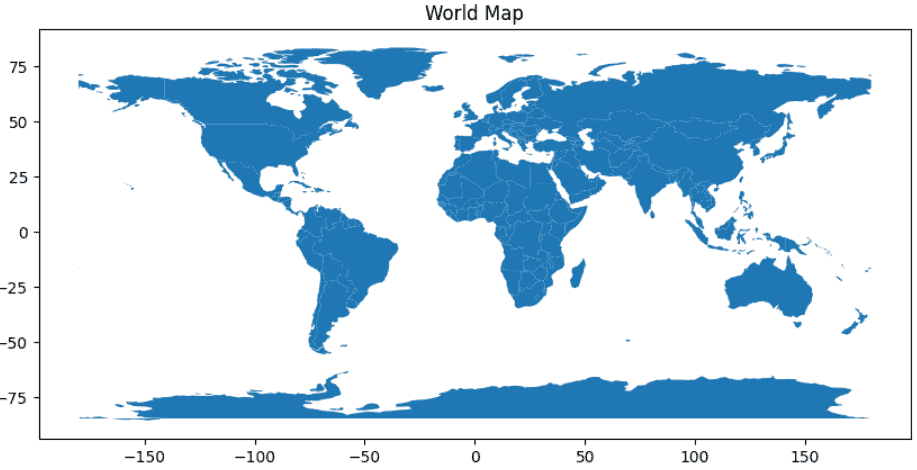
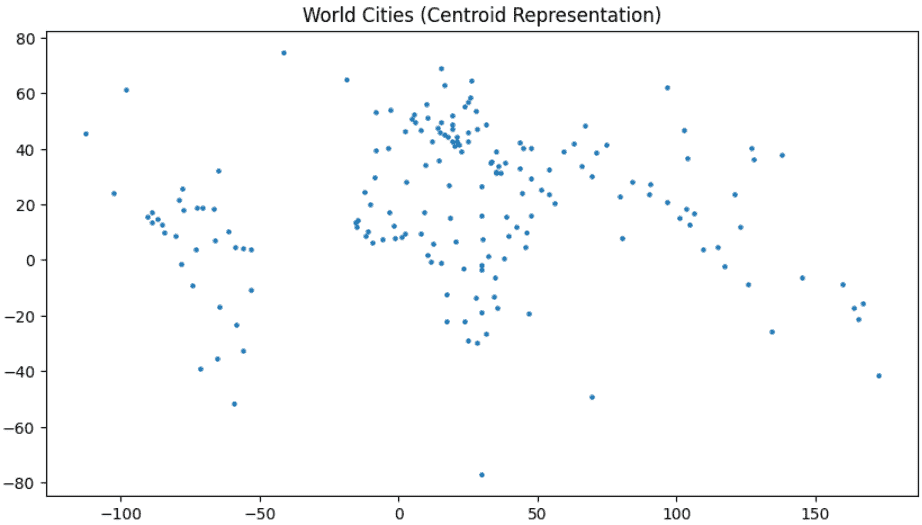
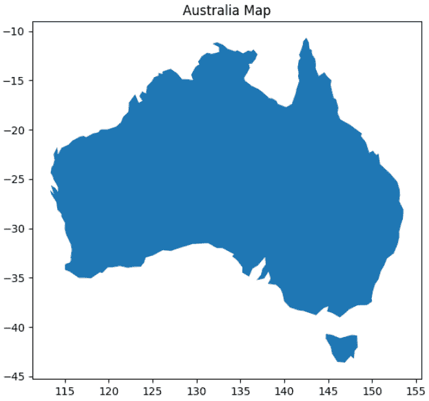
Example: In this example, we visualize multiple built-in geospatial datasets such as world boundaries, USA map, and sample point-based city data using GeoPandas’ plot() function.
world.plot(figsize=(10, 6))
plt.title("World Map")
plt.show()

usa = world[world["name"] == "United States of America"]
usa.plot(figsize=(8, 6))
plt.title("USA Map")
plt.show()

cities = world.copy()
cities["geometry"] = cities.centroid
cities.plot(figsize=(10, 6), markersize=5)
plt.title("World Cities (Centroid Representation)")
plt.show()

melbourne = world[world["name"] == "Australia"]
melbourne.plot(figsize=(8, 6))
plt.title("Australia Map")
plt.show()
Output:
Four geospatial visualizations will be generated: World map, USA map, centroid-based city points, and Australia map.
Combining Countries and Cities on One Map
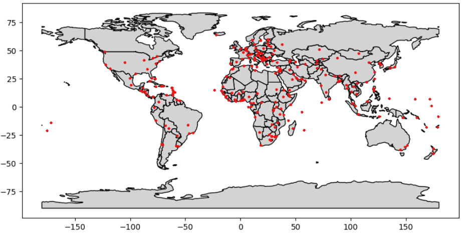
Overplotting means drawing multiple geospatial layers on the same map to add more context. Here, we plot world country boundaries and city locations together to better understand how points (cities) are distributed across regions.
Syntax:
GeoDataFrame.plot(ax=ax)
Example: In this example, we load world boundaries and city datasets directly from online sources. Then we use Matplotlib axes (ax) to overlay both layers on a single map for combined visualization.
world = gpd.read_file("https://naturalearth.s3.amazonaws.com/110m_cultural/ne_110m_admin_0_countries.zip")
cities = gpd.read_file("https://naturalearth.s3.amazonaws.com/110m_cultural/ne_110m_populated_places.zip")

fig, ax = plt.subplots(figsize=(10, 6))
world.plot(ax=ax, color="lightgray", edgecolor="black")
cities.plot(ax=ax, color="red", markersize=5)

plt.show()
Output:
Explanation:
- gpd.read_file(...) loads geospatial datasets directly from a URL.
- world.plot(ax=ax) draws country boundaries as the base map.
- cities.plot(ax=ax) overlays city points on the same axes.
- ax ensures both plots are drawn on a single shared map.
Map Projections with Point Overlay
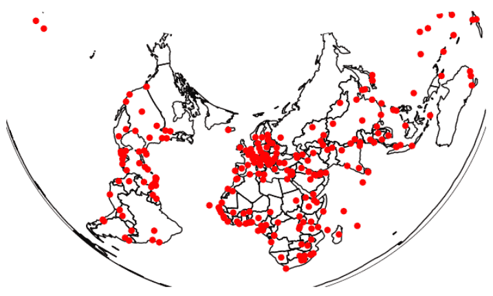
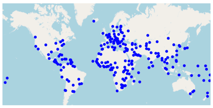
Map projections help convert the Earth’s curved surface into a flat map. We use different projections like Albers Equal Area and Web Mercator to visualize spatial data more accurately. City points are then overlaid on country boundaries for better interpretation.
Syntax:
gplt.polyplot(data, projection=...)
gplt.pointplot(data, ax=ax)
Example: In this example, we load world boundaries and city datasets from online sources. Then we plot country polygons and overlay city locations using a shared axis.
import geoplot.crs as gcrs

world = gpd.read_file("https://naturalearth.s3.amazonaws.com/110m_cultural/ne_110m_admin_0_countries.zip")
cities = gpd.read_file("https://naturalearth.s3.amazonaws.com/110m_cultural/ne_110m_populated_places.zip")

ax = gplt.polyplot(world, projection=gcrs.AlbersEqualArea())
gplt.pointplot(
    cities,
    ax=ax,
    color="red"
)

ax = gplt.webmap(world, projection=gcrs.WebMercator())
gplt.pointplot(
    cities,
    ax=ax,
    color="blue"
)
Output:
World map with city locations displayed using Albers Equal Area and Web Mercator projections
Explanation:
- polyplot() draws country boundaries.
- pointplot() overlays city points.
- projection= changes map distortion behavior.
- color sets point color safely (no errors).
- Removing scale avoids length mismatch errors.
Choropleth Map
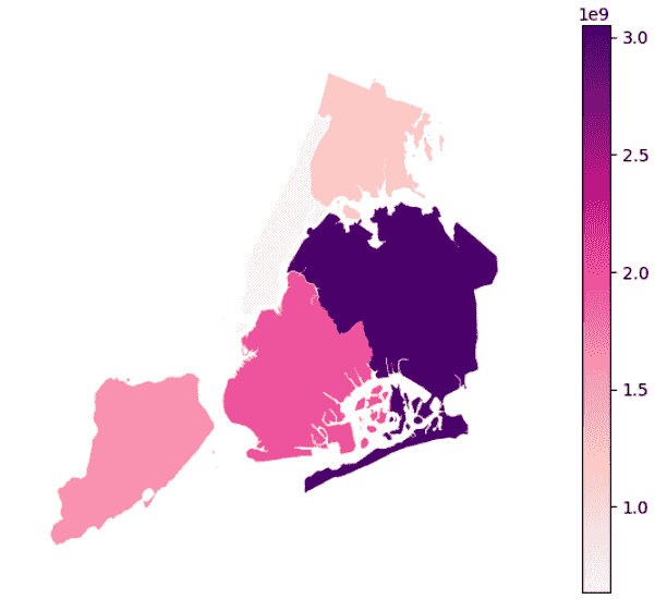
A choropleth map represents geographic regions using different colors based on a numeric attribute. It is commonly used to visualize patterns such as population, area, or density across regions like states or boroughs. Darker or lighter shades represent variation in values across polygons.
Syntax:
gplt.choropleth(data, hue=..., projection=..., cmap=..., legend=True)
Example: In this example, we load NYC borough boundary data and visualize it using a choropleth map. The area of each borough is represented using a color gradient with a legend for interpretation.
boroughs = gpd.read_file(gplt.datasets.get_path('nyc_boroughs'))
gplt.choropleth(
    boroughs,
    hue='Shape_Area',
    projection=gcrs.AlbersEqualArea(),
    cmap='RdPu',
    legend=True
)
Output:
Explanation:
- choropleth() colors regions based on a numeric column.
- hue='Shape_Area' defines the variable used for coloring.
- cmap='RdPu' controls the color gradient.
- legend=True shows the color scale for interpretation.
- AlbersEqualArea() preserves area accuracy for better comparison.
Advanced Choropleth Mapping with Classification
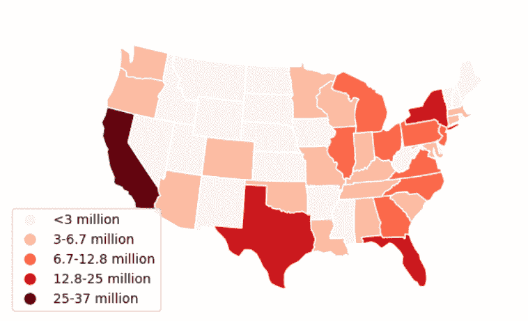
Choropleth maps can be enhanced using classification schemes to group continuous data into meaningful categories. This makes patterns easier to interpret, especially for large datasets. Libraries like mapclassify help apply statistical methods such as Fisher Jenks to divide data into classes.
Syntax:
gplt.choropleth(
data,
hue=...,
scheme=...,
legend=True,
legend_labels=...
)
Example: In this example, we load USA spatial data and classify population values into meaningful groups using the Fisher Jenks algorithm. The map is then visualized using a choropleth with a categorized legend.
import mapclassify as mc

contiguous_usa = gpd.read_file(gplt.datasets.get_path('contiguous_usa'))
scheme = mc.FisherJenks(contiguous_usa['population'], k=5)

gplt.choropleth(
    contiguous_usa,
    hue='population',
    projection=gcrs.AlbersEqualArea(),
    edgecolor='white',
    linewidth=1,
    cmap='Reds',
    legend=True,
    legend_kwargs={'loc': 'lower left'},
    scheme=scheme,
    legend_labels=[
        '<3 million', '3-6.7 million', '6.7-12.8 million',
        '12.8-25 million', '25-37 million'
    ]
)
Output:
Explanation:
- FisherJenks groups continuous population data into 5 meaningful classes.
- scheme applies this classification to the choropleth.
- hue='population' determines the color mapping variable.
- cmap='Reds' sets the color gradient.
- legend_labels customizes category names in the legend.
- AlbersEqualArea() ensures area accuracy in visualization.
KDE Plot
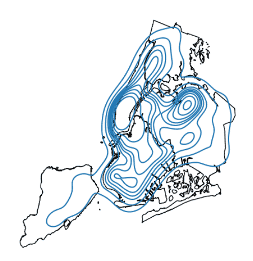
Kernel Density Estimation (KDE) is used to visualize the density of point data over a geographic area. Instead of showing individual points, it creates smooth density regions that highlight where events are concentrated. It is widely used in spatial analysis for detecting hotspots.
Syntax:
gplt.kdeplot(data, ax=ax)
Example: In this example, we load NYC borough boundaries and collision point data. We first plot the borough map and then overlay a KDE plot to visualize areas with high collision density.
boroughs = gpd.read_file(gplt.datasets.get_path('nyc_boroughs'))
collisions = gpd.read_file(gplt.datasets.get_path('nyc_collision_factors'))

ax = gplt.polyplot(boroughs, projection=gcrs.AlbersEqualArea())
gplt.kdeplot(collisions, ax=ax)
Output:
Explanation:
- kdeplot() estimates spatial density of point data.
- polyplot() provides the base geographic boundary (boroughs).
- KDE highlights regions with higher concentration of events.
- AlbersEqualArea() ensures accurate spatial representation.
- Useful for detecting geographic “hotspots” in data.
