Every database needs to answer a simple question: which event came first? On one machine, a clock answers it. Across many machines, however, there is no single clock to ask. In this article, we will see why wall-clock time fails, how hybrid logical clocks repair it, and what a small simulation shows.
Why Wall-Clock Time Cannot Order Events
Each server has its own clock, and tools such as NTP keep those clocks only roughly aligned. The hybrid logical clock paper calls the maximum difference between two clocks the skew, written as ε. Consequently, a message can leave one machine at 10:00:00.005 and arrive on another machine whose clock already reads 10:00:00.002. The receive event then looks older than the send event.
My own simulation shows how common this is. With five nodes, a mean network delay of 1 ms, and a 10 ms skew bound, 43.9% of messages were stamped out of order by plain physical timestamps. Meanwhile, the hybrid clock produced none.
Two Old Answers, Two Old Problems
Logical Clocks: Order Without Time
Lamport’s logical clocks, introduced in 1978, count events instead of reading a clock. Therefore, they always respect cause and effect. On the other hand, their values say nothing about wall-clock time, so you cannot ask a database for “everything before 10:00”.
TrueTime: Time With Special Hardware
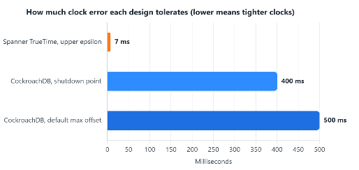
Google Spanner took the opposite route. Its TrueTime API returns an interval instead of a single instant, and the uncertainty ε follows a sawtooth between roughly 1 and 7 ms, according to a talk by Spanner engineer Alex Lloyd. Time masters with GPS receivers or atomic clocks make this possible, and a write simply waits out the uncertainty before it commits. The result is excellent, but the hardware is not something every team can buy.
The Hybrid Idea
Two Numbers Instead of One
In 2014, Kulkarni, Demirbas, and colleagues proposed a hybrid logical clock, or HLC. Each node keeps three values: its physical clock pt, a logical time l, and a small counter c. The value l is the highest physical time the node has seen, either from its own clock or from a message. The counter c only breaks ties when l does not move.
Two properties make the design practical. First, l never drifts more than ε away from the physical clock. Second, the pair fits into the 64-bit NTP timestamp format, and HLC only reads the physical clock without changing it. As a result, it can run next to NTP without conflict.
A Small Example You Can Run
The script below needs only Python 3. It simulates two nodes with fake clocks, where node B runs 100 ms behind node A. B receives a message from A and still produces timestamps that sort after it. Later, when B’s own clock passes A’s time, the counter resets.
cat > hlc_demo.py <<'PY'
class HLC:
    def __init__(self, clock):
        self.clock, self.l, self.c = clock, 0, 0

    def tick(self):
        """Local or send event."""
        pt = self.clock()
        if pt > self.l:
            self.l, self.c = pt, 0
        else:
            self.c += 1
        return (self.l, self.c)

    def receive(self, ml, mc):
        """Receive event carrying the sender's timestamp (ml, mc)."""
        pt = self.clock()
        new_l = max(self.l, ml, pt)
        if new_l == self.l == ml:
            self.c = max(self.c, mc) + 1
        elif new_l == self.l:
            self.c += 1
        elif new_l == ml:
            self.c = mc + 1
        else:
            self.c = 0
        self.l = new_l
        return (self.l, self.c)

# Fake wall clocks in milliseconds: B runs 100 ms behind A.
now = {"A": 1000, "B": 900}
a = HLC(lambda: now["A"])
b = HLC(lambda: now["B"])

sent = a.tick()
print("A sends at          ", sent)
print("B receives at       ", b.receive(*sent))
print("B local event at    ", b.tick())
now["B"] = 1100
print("B clock catches up  ", b.tick())
PY

python3 hlc_demo.py
The output is deterministic. A sends at (1000, 0), B receives at (1000, 1), B’s next local event is (1000, 2), and finally B reaches (1100, 0) once its own clock overtakes. In other words, B’s slow clock never produces a timestamp earlier than the message it received.
What My Simulation Measured
To see the guarantees in numbers, I ran a seeded simulation. It used five nodes, 10 seconds of activity, 500 events per second per node, and exponentially distributed network delay with a 1 ms mean. Each run delivered 25,000 messages, and clock offsets were drawn within the chosen skew bound. I repeated it for eight skew values. Every timestamp pair was compared, and the HLC never produced an out-of-order message.
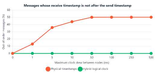
Notably, plain physical timestamps flip about half of all messages once skew is much larger than the network delay. At that point, the sign of the clock offset decides the order, which is close to a coin toss. The table also confirms the key bound: the gap between l and the physical clock stayed below ε in every run.
| Skew bound ε | Largest l minus pt seen | Largest c seen | HLC out-of-order messages |
|---|---|---|---|
| 1 ms | 0.58 ms | 5 | 0 |
| 10 ms | 5.78 ms | 15 | 0 |
| 100 ms | 57.85 ms | 32 | 0 |
| 500 ms | 289.25 ms | 32 | 0 |
One caveat deserves mention. The Retroscope paper reports that c stayed below 10 in its evaluations, whereas my run reached 32. My event rate is high and my timestamps are in microseconds, so the counter grows while a node waits for its slower clock. Therefore, read it as a property of my model, not as a contradiction.
Where HLCs Run in Production
CockroachDB uses HLCs to order transactions. Its documentation says clocks need moderate synchronization, and a node shuts itself down when it drifts too far from at least half of the others. The default maximum offset is 500 ms, and the shutdown point is 80% of it, or 400 ms. MongoDB took a similar path in version 3.6. Its signed $clusterTime is gossiped between nodes, and a SIGMOD 2019 paper describes this causal consistency design as built on hybrid logical clocks.
The Catches
Of course, HLCs are not magic. First, the guarantee is one-way: if event A happened before event B, then A’s timestamp is smaller. The reverse is only approximately true, because concurrent events can be ordered either way. Second, the bounds rely on clocks staying within ε. CockroachDB’s own FAQ explains that serializability holds regardless of skew, but skew beyond the configured offset can break single-key linearizability between causally dependent transactions.
In addition, clock jumps are a real hazard. A node whose clock suddenly leaps past the maximum offset can briefly run unsynchronized before it detects the problem. Hence, monitoring clock offset is part of operating such a database, not an optional extra.
Choosing a Time Strategy
| Approach | Orders cause and effect | Close to wall time | Special hardware |
|---|---|---|---|
| Physical (NTP) | No, once skew exceeds delay | Yes | No |
| Lamport | Yes | No | No |
| Vector clocks | Yes, and detect concurrency | No | No, but they grow with node count |
| HLC | Yes, one-way | Yes, within ε | No |
| TrueTime | Yes, by waiting out ε | Yes, as an interval | GPS and atomic clocks |
Checklist before you rely on HLC timestamps
- Do you know the skew bound ε that your clock sync really delivers?
- Do you alert on clock offset before it reaches a shutdown threshold?
- Can your platform freeze a clock, for example during VM migration?
- Do you need to detect concurrent events, which HLCs cannot do?
- Do all nodes use the same time source and leap-second handling?
What We Have Learned
Physical clocks drift, so wall-clock timestamps can place a received message before its own send. In my simulation, that happened to 43.9% of messages at a 10 ms skew bound. Lamport clocks fix the order but lose the link to real time, while Spanner’s TrueTime keeps both by using GPS and atomic clocks. A hybrid logical clock offers a middle path: a pair of values, l and c, that never goes backwards across messages, stays within ε of the physical clock, and fits into 64 bits. CockroachDB and MongoDB rely on this idea in production. However, the guarantee is one-way, it depends on bounded skew, and it needs clock monitoring. In short, HLCs do not remove time as a dependency, but they make that dependency measurable and manageable.