Data Science

Gradient Boosted Trees for Classification - One of the Best Machine Learning Algorithms

A step by step guide to how Gradient Boosting works in classification trees

Saul Dobilas
March 7, 202112 min read

Machine Learning

Intro

Gradient Boosted Trees is one of my favorite algorithms, and it's been widely used by many Data Scientists. Whether you are building a model for your own project or trying to win a Kaggle competition, it is always worth considering Gradient Boosting.

Gradient Boosting Classification - how model prediction probabilities change after adding more Decision Trees. Image by the author.

In this story, I will take you through the details of how the algorithm actually works and provide Python code resources for you to use in your own projects.

Contents

  • The category of algorithms Gradient Boosted Trees belong to

  • Definitions and fundamentals

  • Example based explanation of Gradient Boosted Trees

  • Python code resources

What category of algorithms does Gradient Boosting belong to?

Gradient Boosting is a tree-based algorithm, which sits under the supervised branch of Machine Learning. Note that it can be used for both classification and regression problems. In this story, however, I will focus on the classification side.

Side note, I have put Neural Networks in a category of their own due to their unique approach to Machine Learning. However, they can be used to solve a wide range of problems, including but not limited to classification and regression. The below chart is interactive so make sure to click👇 on different categories to enlarge and reveal more.

If you enjoy Data Science and Machine Learning, please subscribe to get an email whenever I publish a new story.

Definitions and Fundamentals

To understand how Gradient Boosted Trees are formed, we need to familiarize ourselves with logistic regression and decision tree concepts.

  • Regression Trees - this may sound strange at first, but the Gradient Boost Classification algorithm does not use Classification Trees. Instead, it uses Regression Trees. This is because the target in Gradient Boosted Trees is the residual, not the class label. Don't worry if you are confused about this. It will become clearer once we start going through the example.

  • Residual - it is the difference between the observed value and the estimated value (prediction). We will use residuals for calculating MSE and for tree predictions.

  • MSE (Mean Squared Error) - there are multiple ways to find the best split in the tree node, with MSE being one of the most common approaches used for regression trees. Hence, MSE is what we will use in our algorithm. Note, 'Observed' and 'Predicted' are the actual and model-predicted values for each data record.Residual = (Observed - Predicted).

  • Odds Ratio - it is simply a ratio between the number of events and non-events. Say, if your data contains 3 spam emails and 2 non-spam emails, the odds would be 3:2 (1.5 in decimal notation).

  • Log(odds) - is a natural logarithm of the odds ratio. So if, the odds are 3:2 = 1.5, then log(odds) = log(1.5) = 0.405...

  • Probability vs. odds - it is easy to convert odds to probabilities and vice versa. For example if, the odds are 3:2, then the probability is 3/5 = 0.6.You can use the following equations to convert between probability and odds:

  • The probability expressed through log(odds) - is the final piece that we will need for our model calculations:
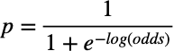
Note, if you want to get a deeper understanding of the above concepts, you can refer to my story about Logistic Regression:

Logistic Regression in Python— A Helpful Guide to How It Works

Gradient Boosted Trees - example-based explanation

First, let me share with you a process map to help you see how each step fits together to produce a Gradient Boosted Trees model.
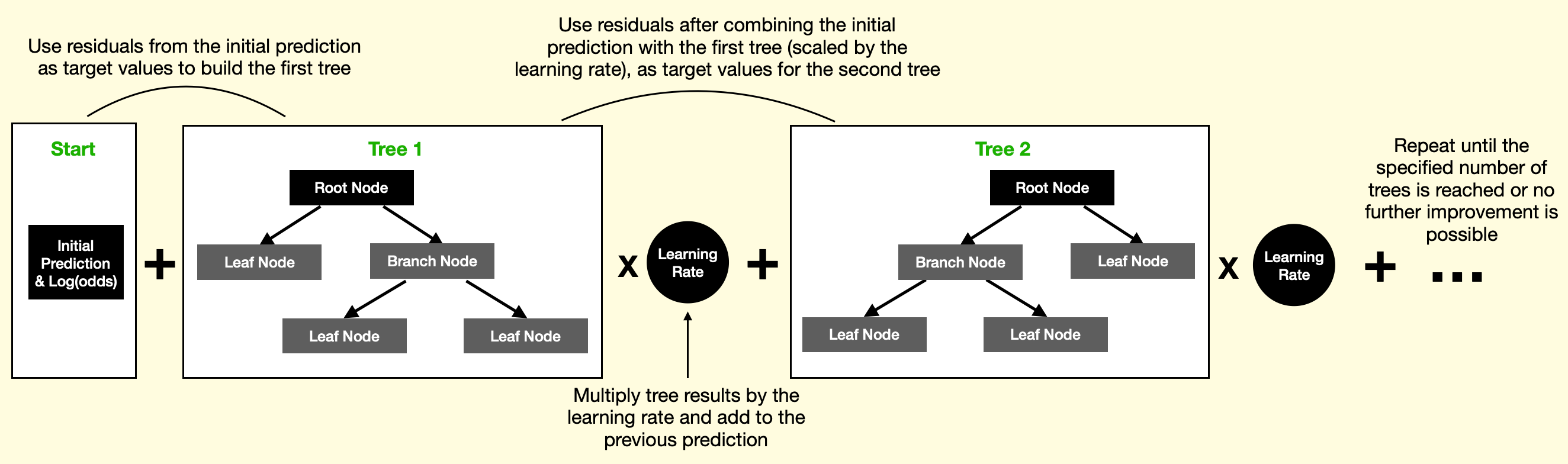
Process map for Gradient Boosted Trees. Image by the author.

Start

First, let's take a look at the data we will use.

We have 9 observations from the Australian weather dataset with 'Wind Gust Speed' and 'Humidity at 3 pm' as our two model features (independent variables). 'Rain Tomorrow Flag' is what we want to predict with our model.

Note, we are using a tiny set of data because we want to make the explanation easier. However, the algorithm works the same with a much larger dataset.

Our data contains 5 observations where Rain Tomorrow = 1 and 4 observations where Rain Tomorrow = 0.

The initial prediction is simply a probability derived from all observations Probability = 5 / 9 = 0.56. Meanwhile, residuals are calculated for each observation separately and, in this case, take one of the two values: Residual = Observed - Predicted = 1 - 0.56 = 0.44 or 0 - 0.56 = -0.56.

Since we are building a classification model, we will also need to calculate log(odds). While the initial prediction is Probability = 0.56 the log(odds) value of the initial leaf is: Log(odds) = log(5/4) = log(1.25) = 0.22. Note that log(odds) from the initial leaf will be used to recalculate residuals after building Tree 1.

Tree 1

Let's now build the first tree. Below are the model hyperparameters that we use for this specific example. I just want to highlight a few of them at this stage, but I will provide the complete Python code in the Python section at the end of this story.

python
model = GradientBoostingClassifier(loss='deviance', # deviance or explonential                               criterion='squared_error', # {'friedman_mse', 'squared_error', 'mse', 'mae'}, default='friedman_mse'                               learning_rate=0.5, # default 0.1                               subsample=1.0, # default=1.0                               random_state=0, # random state for reproducibility                               max_features=None, # number of random features to use sqrt(n_features), default=None                               min_samples_leaf=1, # minimum no of observarions allowed in a leaf                               max_depth=1, # maximum depth of the tree, default=3                               n_estimators=3 # how many trees to build                              )

While the tree's default size has a max depth of 3, we have set it to 1 to make the example simpler. This means that the trees we are building will be decision stumps. In total, our model will contain 3 decision stumps with the learning set to 0.5.

It is important to reiterate that with Gradient Boosting, we are not predicting class labels (rain / no rain) but residuals instead (see below table).

Let's look a the first decision tree (stump) and work out how it's been created.
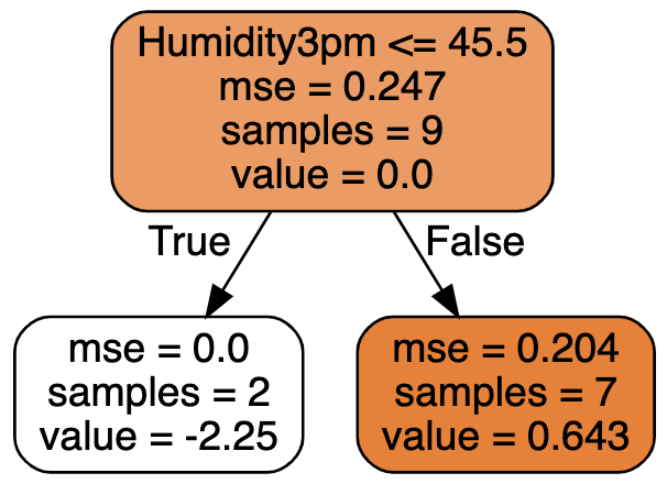
The first decision tree (stump). Image by the author.

The first question to answer is: "Why has the algorithm selected this particular node split (Humidity at 3 pm ≤ 45.5)?"

  • The best split is identified by calculating MSE for every possible split using 'Humidity at 3 pm' and calculating MSE for every possible split using 'Wind Gust Speed.'

  • Then the algorithm compares all of those splits and picks the one with the lowest MSE. You can see the calculation of MSE for the chosen split below.

The second question we need to answer: " What is the purpose of 'value' within the tree, and how is it calculated?"

  • The leaf 'value' is what the algorithm uses to recalculate the residuals, which are then used as a target when building the next tree.

  • 'Value' is calculated with the below formula:

Now let's put all of this knowledge to practice and calculate each of the metrics within the tree:
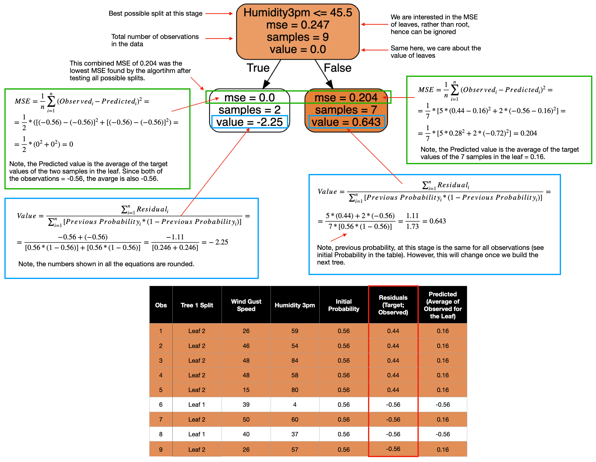
Details of every calculation in the first decision tree (stump). Image by the author.

The last part left to do before moving to Tree 2 is recalculating the residuals (model targets). Following the steps in the process map above, this is what we need to do to recalculate the residuals for each observation:

text
'New Log(odds)' = 'Log(odds) from the initial prediction' + 'Value from Tree 1' * 'Learning Rate'.
text
Obs1 = 0.22 + 0.643 * 0.5 = 0.54 <-- Example for leaf 2Obs6 = 0.22 + -2.25 * 0.5 = -0.91 <-- Example for leaf 1

Note, the calculation above gives us the new log(odds). However, to get new residuals, we first need to convert log(odds) back to probabilities using this formula:

text
New Predicted Probability (Obs1) = 1/(1+e^(-0.54)) = 0.63New Predicted Probability (Obs6) = 1/(1+e^(0.91)) = 0.29
text
Note how the above probabilities are steps in the right direction for both observations.

Finally, we calculate new residuals using the class label and the new predicted probability.

text
New Residual (Obs1) = 1 - 0.63 = 0.37New Residual (Obs6) = 0 - 0.29 = -0.29

Here is a table containing recalculated values for all observations:

One interesting observation is that the new predictions for Obs7 and Obs9 are actually worse than before. This is exactly why we need to build many trees, as having a larger number of trees will lead to improvements in predictions across all observations. You can see this illustrated in the gif image at the beginning of this story.

Tree 2

Now we can use new residuals to build the second tree. Note, I will not list all of the formulas again since those are the same as in Tree 1. However, if you want to attempt calculations yourself, remember to use the new values from a table created post Tree 1.
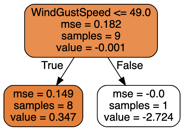
The second decision tree (stump). Image by the author.

The algorithm identified Wind Gust Speed ≤49 as the best node split in the second tree with 8 observations (samples) in leaf 1 and only 1 observation in leaf 2.

Note, when building a larger tree from a big dataset, it is advisable to restrict the minimum number of observations allowed in a leaf to reduce the chance of overfitting.

Since we already know how the leaf values are calculated, let's go straight into finding the new residuals.

text
'New Log(odds) T2' = 'Log(odds) from the initial prediction' + 'Value from Tree 1' * 'Learning Rate' + 'Value from Tree 2' * 'Learning Rate'.
text
Obs1 = 0.22 + 0.643 * 0.5 + 0.347 * 0.5 = 0.72 <-- T1L2-T2L1Obs6 = 0.22 + -2.25 * 0.5 + 0.347 * 0.5 = -0.73 <-- T1L1-T2L1Obs7 = 0.22 + 0.643 * 0.5 + -2.724 * 0.5 = -0.82 <-- T1L2-T2L2
text
As before we convert the above to New Predicted Probabilites
text
Pred Prob T2 (Obs1) = 1/(1+e^(-0.72)) = 0.67Pred Prob T2 (Obs6) = 1/(1+e^(0.73)) = 0.33Pred Prob T2 (Obs7) = 1/(1+e^(0.82)) = 0.31

Then we calculate new residuals and place them in the table below to be used for a target in Tree number 3:

Tree 3...

The same process is repeated when building additional trees until the specified number of trees is reached, or the improvement becomes too small (falls below a certain threshold). For interest, this is what stump number 3 looks like:
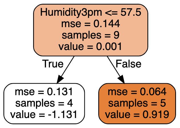
The third decision tree (stump). Image by the author.

Since we restricted our model to only 3 trees, the last part left is to get the final set of predictions by following the above methodology to combine the log(odds). I believe you have got the hang of it by now, so I will not repeat it. Instead, let's jump into the Python code.

Python code resources

Now that you understand how Gradient Boosted Trees work let's build a model using the full set of observations but with the same two features as before. This is so we can generate the below 3D graph to demonstrate model predictions.

Setup

We will use the following data and libraries:

Let's import all the libraries:

python
import pandas as pd # for data manipulationimport numpy as np # for data manipulationfrom sklearn.model_selection import train_test_split # for splitting the data into train and test samplesfrom sklearn.metrics import classification_report # for model evaluation metricsfrom sklearn.ensemble import GradientBoostingClassifierimport plotly.express as px  # for data visualizationimport plotly.graph_objects as go # for data visualization

Then we get the Australian weather data from Kaggle, which you can download following this link: https://www.kaggle.com/jsphyg/weather-dataset-rattle-package.

We ingest the data and derive a few new variables for usage in the model.

python
# Set Pandas options to display more columnspd.options.display.max_columns=50# Read in the weather data csvdf=pd.read_csv('weatherAUS.csv', encoding='utf-8')# Drop records where target RainTomorrow=NaNdf=df[pd.isnull(df['RainTomorrow'])==False]# For other columns with missing values, fill them in with column meandf=df.fillna(df.mean())# Create a flag for RainToday and RainTomorrow, note RainTomorrowFlag will be our target variabledf['RainTodayFlag']=df['RainToday'].apply(lambda x: 1 if x=='Yes' else 0)df['RainTomorrowFlag']=df['RainTomorrow'].apply(lambda x: 1 if x=='Yes' else 0)# Note, these are the 9 observations we used in the example in this story#df9 = pd.concat([df[df['RainTomorrowFlag']==1].sample(5, random_state=40),                 #df[df['RainTomorrowFlag']==0].sample(4, random_state=40)])# Show a snaphsot of datadf
A snippet of Kaggle&#039;s Australian weather data with some modifications. Image by the author.
A snippet of Kaggle's Australian weather data with some modifications. Image by the author.

Model training

Next, we define a function to be used for model training and run the model to produce the results:

  • Step 1— split data into train and test samples

  • Step 2— set model parameters and train (fit) the model

  • Step 3— predict class labels on train and test data using our model

  • Step 4— generate model summary statistics

  • Step 5— run the model and display the results

python
def model_training(X, y, n_trees):    ##### Step 1 - Create training and testing samples    X_train, X_test, y_train, y_test = train_test_split(X, y, test_size=0.2, random_state=0)    ##### Step 2    # Set model and its parameters    model = GradientBoostingClassifier(loss='deviance', #deviance or explonential                               criterion='squared_error', # {'friedman_mse', 'squared_error', 'mse', 'mae'}, default='friedman_mse'                               learning_rate=0.1, # default 1.0                               subsample=1.0, #default=1.0                               random_state=0, # random state for reproducibility                               max_features='sqrt', # number of random features to use sqrt(n_features)                               min_samples_leaf=1000, # minimum no of observarions allowed in a leaf                               max_depth=3, # maximum depth of the tree                               n_estimators=n_trees # how many trees to build                              )    # Fit the model    clf = model.fit(X_train, y_train)    ##### Step 3    # Predict class labels on training data    pred_labels_tr = model.predict(X_train)    # Predict class labels on a test data    pred_labels_te = model.predict(X_test)    ##### Step 4 - Model summary    # Basic info about the model    print('*************** Tree Summary ***************')    print('No. of classes: ', clf.n_classes_)    print('Classes: ', clf.classes_)    print('No. of features: ', clf.n_features_in_)    print('No. of Estimators: ', len(clf.estimators_))    print('--------------------------------------------------------')    print("")    print('*************** Evaluation on Test Data ***************')    score_te = model.score(X_test, y_test)    print('Accuracy Score: ', score_te)    # Look at classification report to evaluate the model    print(classification_report(y_test, pred_labels_te))    print('--------------------------------------------------------')    print("")    print('*************** Evaluation on Training Data ***************')    score_tr = model.score(X_train, y_train)    print('Accuracy Score: ', score_tr)    # Look at classification report to evaluate the model    print(classification_report(y_train, pred_labels_tr))    print('--------------------------------------------------------')    return clf, X_test, y_test##### Step 5 - Select data and call the above function  # Select data for modellingX=df[['WindGustSpeed', 'Humidity3pm']]y=df['RainTomorrowFlag'].values# Train the model and show the resulsclf, X_test, y_test = model_training(X, y, n_trees=500)

These are the model evaluation metrics the above function returns.
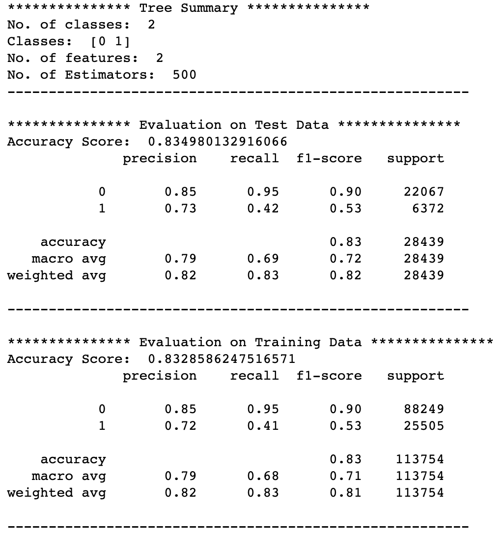
Gradient Boosted Trees - model results. Image by the author.

Finally, you can use the below function to generate the 3D graph shown above.

python
def Plot_3D(X, X_test, y_test, clf, x1, x2, mesh_size, margin, xe, ye, ze):    # Specify a size of the mesh to be used    mesh_size=mesh_size    margin=margin    # Create a mesh grid on which we will run our model    x_min, x_max = X.iloc[:, 0].fillna(X.mean()).min() - margin, X.iloc[:, 0].fillna(X.mean()).max() + margin    y_min, y_max = X.iloc[:, 1].fillna(X.mean()).min() - margin, X.iloc[:, 1].fillna(X.mean()).max() + margin    xrange = np.arange(x_min, x_max, mesh_size)    yrange = np.arange(y_min, y_max, mesh_size)    xx, yy = np.meshgrid(xrange, yrange)    # Calculate predictions on grid    Z = clf.predict_proba(np.c_[xx.ravel(), yy.ravel()])[:, 1]    Z = Z.reshape(xx.shape)    # Create a 3D scatter plot with predictions    fig = px.scatter_3d(x=[], y=[], z=[],                         width=600, height=600)    # Set figure title and colors    fig.update_layout(#title_text="Scatter 3D Plot with Gradient Boost Prediction",                      paper_bgcolor = 'white',                      scene_camera=dict(up=dict(x=0, y=0, z=1),                                         center=dict(x=-0.1, y=0, z=-0.18),                                        eye=dict(x=xe, y=ye, z=ze)),                      scene = dict(xaxis=dict(title=x1,                                              backgroundcolor='white',                                              color='black',                                              gridcolor='#f0f0f0',                                              title_font=dict(size=10),                                              tickfont=dict(size=10),                                             ),                                   yaxis=dict(title=x2,                                              backgroundcolor='white',                                              color='black',                                              gridcolor='#f0f0f0',                                              title_font=dict(size=10),                                              tickfont=dict(size=10),                                              ),                                   zaxis=dict(title='Probability of Rain Tomorrow',                                              backgroundcolor='lightgrey',                                              color='black',                                               gridcolor='#f0f0f0',                                              range=[0.0, 1.0],                                              title_font=dict(size=10),                                              tickfont=dict(size=10),                                              )))    # Update marker size    fig.update_traces(marker=dict(size=1))    # Add prediction plane    fig.add_traces(go.Surface(x=xrange, y=yrange, z=Z, name='Gradient Boost Prediction',                              colorscale='Turbo',                              #colorscale=['darkblue', 'blue'],                              reversescale=True,                              showscale=False,                               contours = {"z": {"show": True, "start": 0.5, "end": 0.9,                                                 "size": 0.5, "color":"white"}}))    fig.show()    fig.update_layout(margin=dict(l=0, r=0, t=1, b=1)                     )    return fig##### Call the above function to generate a graphfig = Plot_3D(X, X_test, y_test, clf, x1='WindGustSpeed', x2='Humidity3pm', mesh_size=1, margin=10,                   xe=-1.7, ye=-1.5, ze=0.4)

Conclusion

Although this story is quite long and with many details, the Gradient Boost algorithm is one of the most important ones to understand for a Data Scientist. I sincerely hope you had fun reading it and that there is no more mystery left behind this algorithm for you.

Cheers! 👏 Saul Dobilas


Also, here are some resources on alternative algorithms if you found this article interesting.

AdaBoost Machine Learning Algorithm: How to Improve Performance of Hard to Predict Cases

Naive Bayes Classifier - How to Successfully Use It in Python?

Related Articles