K-Means Clustering - A Comprehensive Guide to Its Successful Use in Python
Explanation of K-Means algorithm with a Python demonstration on real-life data
Machine Learning
K-Means Clustering - A Comprehensive Guide to Its Successful Use in Python
Intro
If you want to be a successful Data Scientist, it is essential to understand how different Machine Learning algorithms work.
This story is part of the series that explains the nuances of each algorithm and provides a range of Python examples to help you build your own ML models.
The story covers the following topics:
The category of algorithms that K-Means belongs to
An explanation of how the K-Means algorithm works
K-Means limitations and what to do about it
Python example on how to perform K-Means Clustering
What category of algorithms does K-Means belong to?
As a Data Scientist, you will know quite well that it is almost impossible to count and classify all the different Machine Learning algorithms. That is partly because there are so many of them. Simultaneously, they extend across multiple categories (e.g., Neural Networks can be used to solve a wide range of problems, including classification and regression, so I have put them in their own category).
Nevertheless, I have attempted to gather information about some of the most commonly used ones, which you can see in the interactive sunburst chart below. Make sure to click👇 on different categories to enlarge and reveal more.
As for K-Means, it is part of the Unsupervised Machine Learning techniques falling into the group of Clustering algorithms. These are frequently used to group (cluster) customers, objects, or other items based on the similarity of chosen characteristics (attributes).
If you enjoy Data Science and Machine Learning, please subscribe to get an email whenever I publish a new story.
How does the K-Means algorithm work?
K-Means is one the most well-known and most commonly used algorithms due to its simplicity and speed. Although, at the same time, it has some limitations (more on that later).
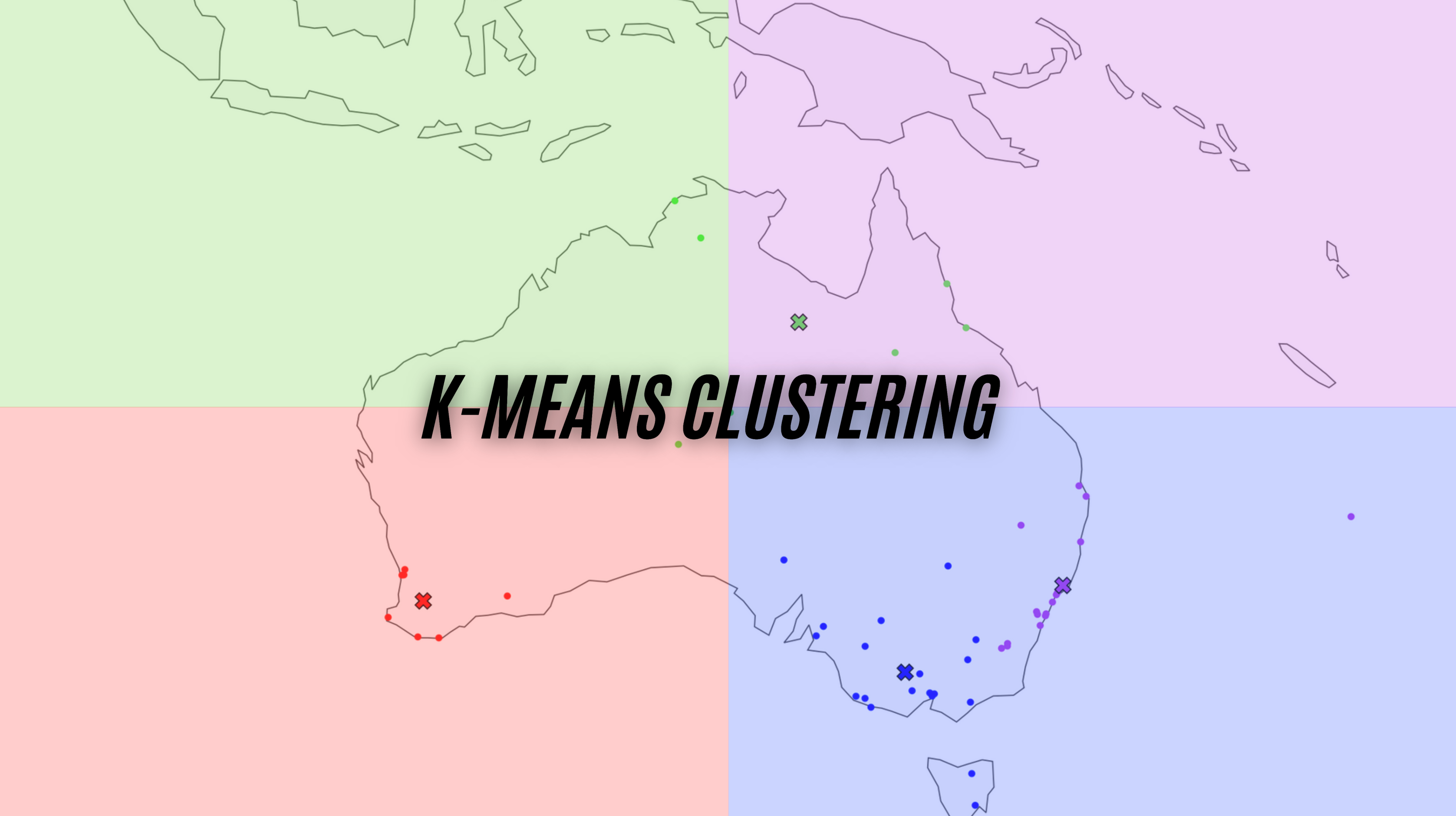
It is designed to make use of a few straightforward steps that are repeated through multiple iterations. You can refer to the below gif for visual explanation while going through the steps listed below.
The first step for the algorithm is to initialize a defined number of centroids (denoted as X's in the chart).
The distance between each point (vector) and each centroid is calculated, and then points are assigned to the nearest centroid.
Each centroid is then assigned a new position based on the mean of all the points (vectors) in the same group (cluster).
The process then repeats with points re-assigned based on new centroid positions and a new mean calculated, leading to new positions for centroids.
The iterations continue until the centroids no longer change their position or the defined number of max iterations is reached.
K-Means limitations and what to do about it
Defining the number of clusters
Before you start the clustering process with K-Means, you need to define how many clusters you want to have. If you have a simple data set with only 2 or 3 dimensions, you can plot the data and visually analyze it to decide the most appropriate number of clusters.
However, that is not ideal, especially if you have a much higher number of attributes (dimensions). To help decide on the appropriate number of clusters, you can employ the "elbow" method. For this, you run K-Means clustering multiple times, trying a different number of clusters each time, and record the value of WCSS (Within Cluster Sum of Squares). Note, WCSS is called "inertia" in sklearn.
Once you have done that, plot the WCSS value onto a line chart like the one below (Python section later in the article will show exact steps on how to perform this):
WCSS reduces as you introduce more clusters. However, after a certain point, the reduction in WCSS is only minimal, which indicates that splitting clusters into more clusters is not needed as the points within them are more similar than different.
In the above case, the "elbow" is around k=3 or k=4. Hence, 3 or 4 is the max number of clusters you want to have. Note, I used this chart to decide on 4 clusters for the Australian city gif you saw earlier.
Centroid initialization
The basic K-Means algorithm initializes centroids randomly. Hence, the result may differ based on the initial position of your centroids and may not be optimal.
To fix this, you can employ the following tactics:
Initialize centroids multiple times and pick the best run (lowest WCSS)
Use smart initialization available with k-means++
Both of the above are implemented as default settings in sklearn's KMeans algorithm.
Distance-based algorithm
K-Means uses the euclidean distance between different points in space (vectors) to identify which ones belong together. Because of that, you also need to be aware of the following:
You can only use numerical attributes in the K-Means algorithm. If you want to use categorical ones for your clustering, you will first need to convert them to numerical. There are multiple ways of doing this, such as using sklearn's Ordinal Encoder or similar methods.
Be mindful of the scale and distribution of the attributes that you are using in your clustering. You may want to first exclude outliers by removing them or introducing "range caps." You may also want to use Power Transformation or Min-Max scaling to transform and fit the distribution into the same range for each of your attributes.
Finally, depending on the type of your data and your use case, you may prefer to use a density-based algorithm instead of a distance-based one.
K-Means in Python using real-world data
Setup
We will use the following data and libraries:
Scikit-learn library to perform K-Means clustering
Plotly and Matplotlib for data visualizations
Pandas for data manipulation
Geopy, Progressbar, and Time for collecting Australian city coordinates
Let's import all the libraries:
Then we get the Australian weather data from Kaggle, which you can download following this link: https://www.kaggle.com/jsphyg/weather-dataset-rattle-package.
We ingest the data and derive a few new variables, such as Location2, which has the right format to extract city coordinates using Geopy.
Since our original data only contains location (city) names and not coordinates, we will use Geopy's Nominatim to get those coordinates. Note that we add a sleep time of 1 second between each call not to overload the server.
And this is the snippet of what we get in return:
We can also plot it on the map:
K-Means clustering
As described earlier, the first thing we need to do is to figure out how many clusters we want. For that, we use the "elbow" method. Here is the code:
Say we could not decide between 3 or 4 clusters, so we perform clustering and visualize both options:
The above code produces the following summary:
Then, we attach cluster labels back to the df_loc data frame and plot the results on the map. Note, you will need to change from ['Clust3'] to ['Clust4'], add extra color, and point to model4 to generate the second plot.
3 clusters:
4 clusters:
Conclusion
Clustering is rarely the end of your analysis. In many cases, it is just the beginning.
For example, you may want to build a supervised classification model to predict the chance of rain tomorrow using the Australian weather data. City location may prove to be an important feature since the climate in nearby places tends to be similar. Hence, you may decide to use the above clusters as one of the features you feed into your prediction model.
In the end, whatever your goal is, I hope this story helped you to get a better understanding of K-Means clustering and that you will feel confident to try it out yourself.
Feel free to let me know if you have any questions or suggestions!
Cheers! 👏 Saul Dobilas
I also picked some additional reading you may enjoy:
HAC: Hierarchical Agglomerative Clustering. Is It Better Than K-Means?
BBN: Bayesian Belief Networks - How to Build Them Effectively in Python?