HAC: Hierarchical Agglomerative Clustering. Is It Better Than K-Means?
A detailed look into the HAC algorithm together with Python code and several useful charts
Machine Learning
HAC: Hierarchical Agglomerative Clustering - Is It Better Than K-Means?
Intro
If you want to be a successful Data Scientist, it is essential to understand how different Machine Learning algorithms work.
This story is part of the series that explains the nuances of each algorithm and provides a range of Python examples to help you build your own ML models.
The story covers the following topics:
The category of algorithms Hierarchical Agglomerative Clustering (HAC) belongs to.
Details of how the HAC algorithm works.
Python example, which uses HAC to cluster Australian cities.
What category of algorithms does Hierarchical Agglomerative Clustering belong to?
The answer is hidden in its name. Since HAC is a clustering algorithm, it sits under the Unsupervised branch of Machine Learning.
Unsupervised techniques, in particular clustering, are often used for segmentation analysis or as a starting point in more complex projects that require an understanding of similarities between data points (e.g., customers, products, behaviors).
The below chart is my attempt to categorize a wide range of different algorithms. In many cases, an algorithm can be used to solve multiple types of problems. E.g., I placed Neural Networks in a category of their own due to their unique approach to Machine Learning. However, NNs can be used in a wide array of problems such as classification, regression, or as a component of reinforcement learning.
The below graph is interactive, so please click on different categories to enlarge and reveal more👇 .
If you enjoy Data Science and Machine Learning, please subscribe to get an email whenever I publish a new story.
How does the Hierarchical Agglomerative Clustering (HAC) algorithm work?
The basics
HAC is not as well-known as K-Means, but it is quite flexible and often easier to interpret. It uses a "bottom-up" approach, which means that each observation starts in its own cluster, and pairs of clusters are merged as one moves up the hierarchy.
To help illustrate this, I have created a few graphs. The first one demonstrates how the algorithm merges closest points one step at a time until there is only one cluster remaining.
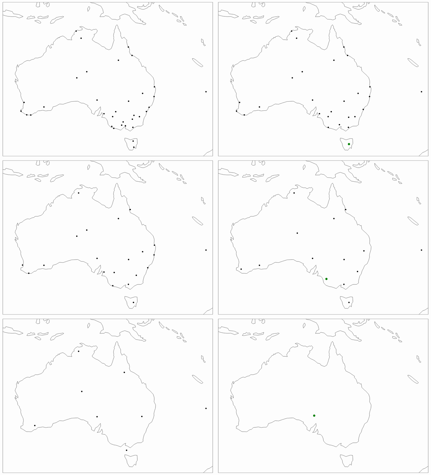
Note, the above implementation of HAC uses 'average' linkage, which I will explain later in this section.
The second graph is known as a Dendrogram. It gives the full picture of the path taken, moving from all individual points (bottom of the graph) to one single point/cluster (top of the graph).
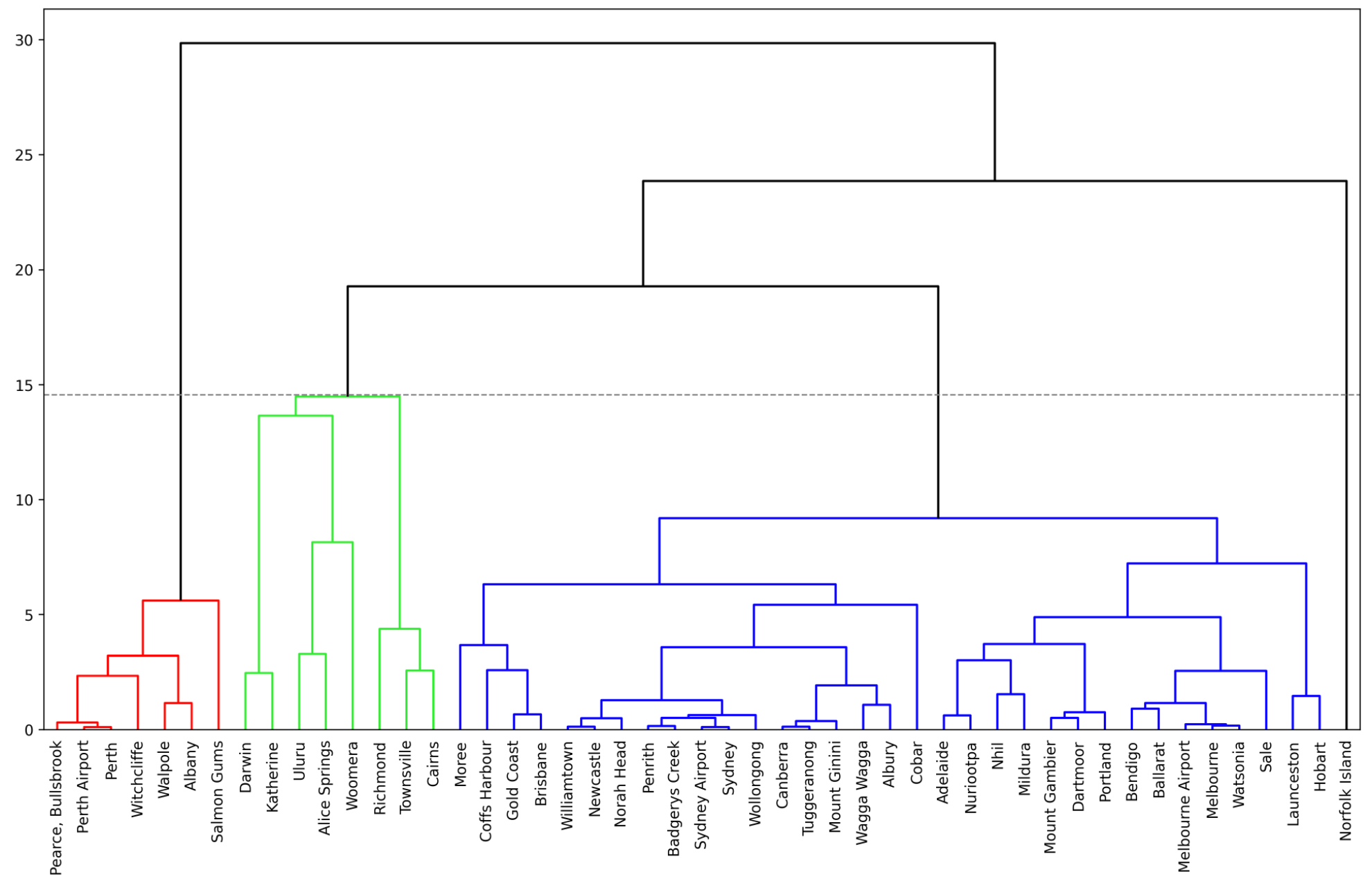
Note, I have added a dotted horizontal line to indicate the number of clusters I have selected. In general, a good rule of thumb is to identify the largest section within the y-axis where you do not have vertical lines intersected by any horizontal lines. Let me explain further.
The value on the y-axis is the measure of closeness between points/clusters. The horizontal lines denote places where those points/clusters are being merged.
The above graph indicates that you may want to consider having 2 clusters since the largest distance with no cluster mergers is between 24 and 30 (30–24=6).
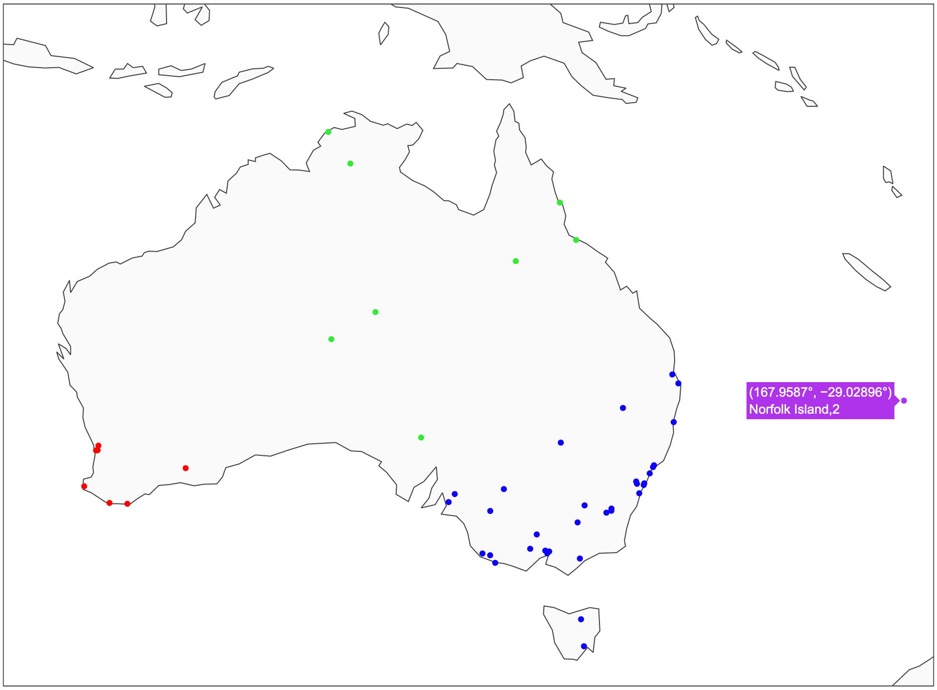
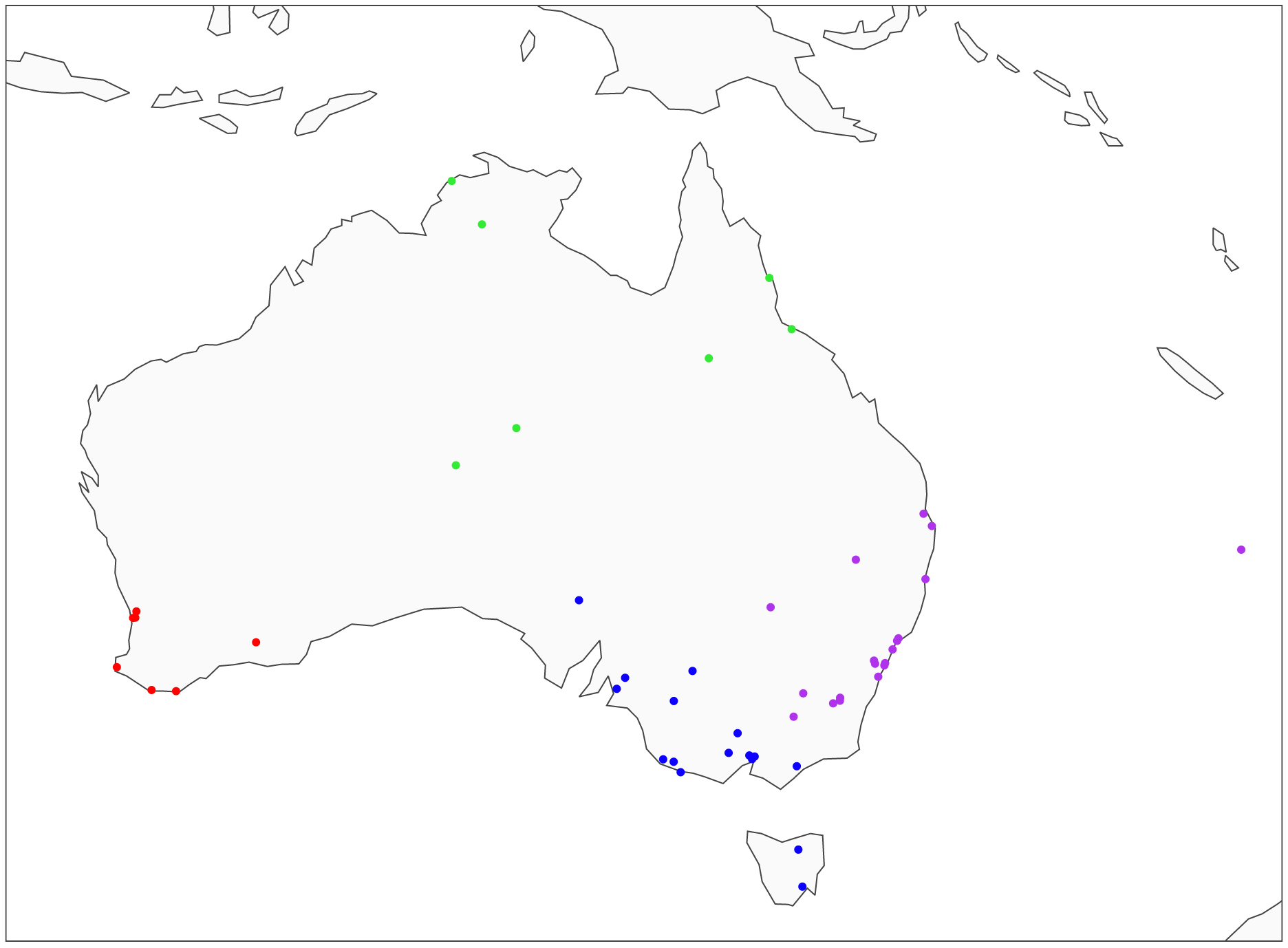
However, in this case, I decided to choose 4 clusters instead, which is a slightly less optimal solution (approx. 19.5–14.5=5). Hence, my clusters are red, bright green, blue, and Norfolk Island that sits in the corner on its own.
Here is what the clusters look like on a map:
Linkage types
There are multiple ways to link the points together. I used 'average' linkage in the above example since it is easy to illustrate and understand. However, it is important to familiarize yourself with other linkage types too. Note, Python section at the end of this article will show you how to specify which linkage method you want to use.
'Average': uses the average of the distances of each observation of the two sets, i.e., finds the mid-point between observations (as shown in the graphs).
'Single': uses the minimum of the distances between all observations of the two sets, i.e., looks for the closest point within the cluster of points at that stage (instead of cluster mid-point used in 'average').
'Complete' or 'Maximum': uses the maximum distance between all observations of the two sets. E.g., if the point is closer to the farthest point of Cluster A than the farthest point of Cluster B, then such a point would be added to Cluster A.
'Ward': minimizes the variance of the clusters being merged. This is very similar to minimizing Within Cluster Sum of Squares (WCSS) used by K-Means.
'Ward' linkage is typically the one that is used most often. It is also the default option for sklearn's implementation of HAC, which we will explore in the Python section below.
HAC advantage over K-Means clustering
The attractive part of using HAC is the ability to analyze dendrogram, which provides an insight into the similarity level between any two data points.
It only takes one glance at a dendrogram to see that Pearce, Bullsbrook is very 'distant' from Norfolk Island, while Sydney and Sydney Airport are quite close together. While this is fairly obvious given our location data, it becomes very beneficial when we use more abstract attributes.
In general, you can generate very similar clusters using HAC and K-Means, but having the ability to see the path of each data point, makes HAC more useful in analyzing similarities and differences between individual data points or clusters.

Hierarchical Agglomerative Clustering (HAC) in Python using Australian city location data
Setup
We will use the following data and libraries:
Scikit-learn library to perform HAC clustering
Scipy library to create a dendrogram
Plotly and Matplotlib for data visualizations
Pandas for data manipulation
Geopy, Progressbar, and Time for collecting Australian city coordinates
Let's import all the libraries:
Then we get the Australian weather data from Kaggle, which you can download following this link: https://www.kaggle.com/jsphyg/weather-dataset-rattle-package.
We ingest the data and derive a few new variables, such as Location2, which has the right format to extract city coordinates using Geopy.
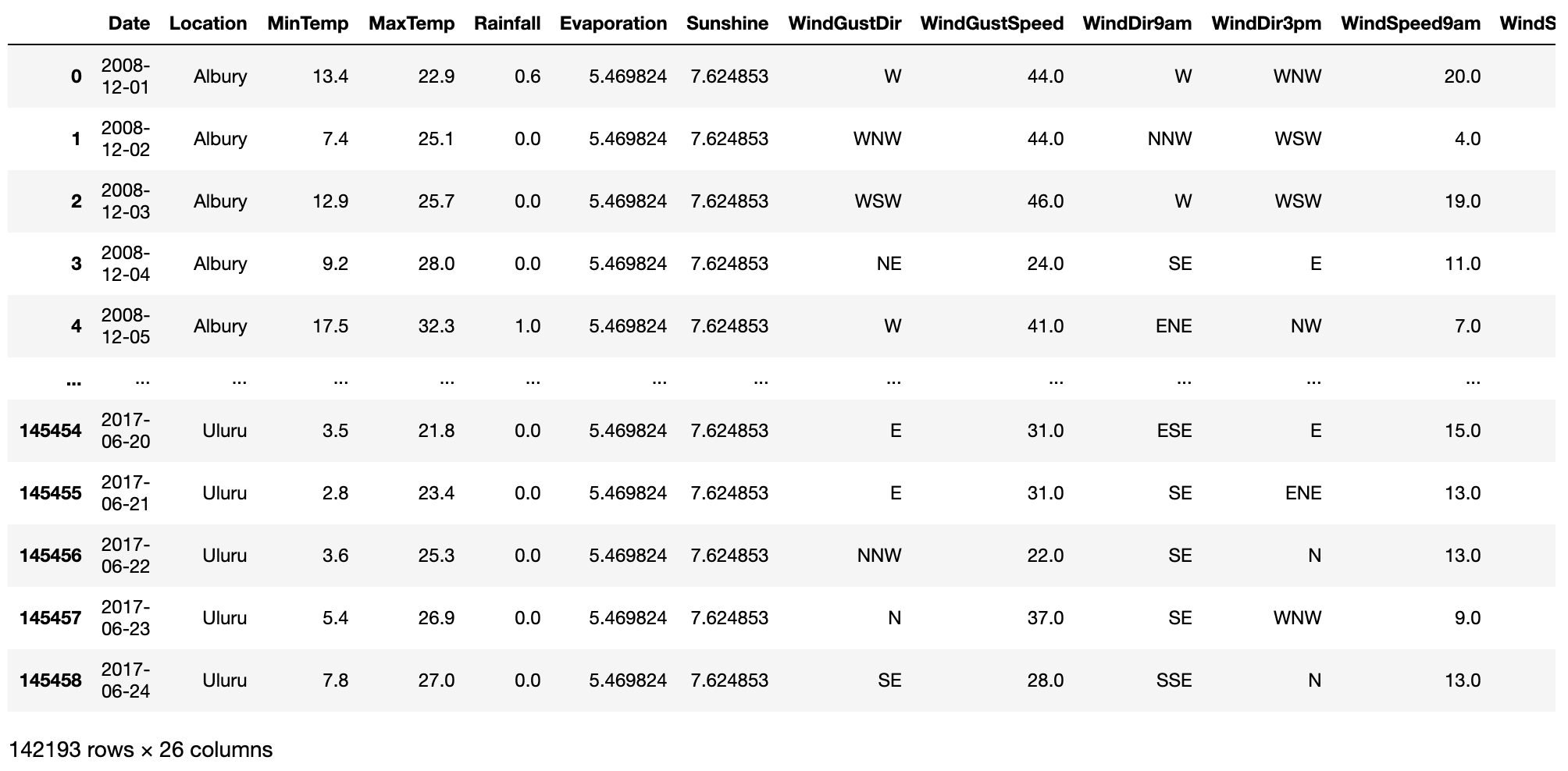
Since our original data only contains location (city) names and not coordinates, we will use Geopy's Nominatim to get those coordinates. Note that we add a sleep time of 1 second between each call not to overload the server.
And this is the snippet of what we get in return:
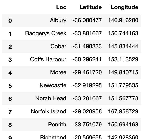
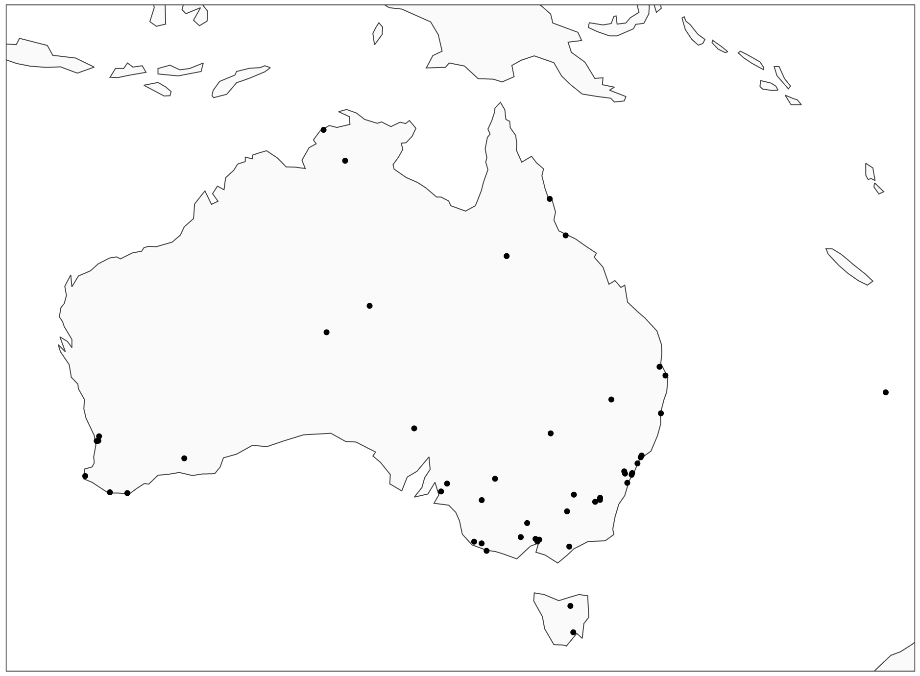
Let's plot the cities on a map:
HAC clustering - dendrogram
To decide on the number of clusters, we will first draw a dendrogram like the one we have analyzed earlier. Note, we will draw two of them, one using 'average' linkage and another using 'ward' linkage so you can see the difference in the results.
Average linkage:
Ward linkage:
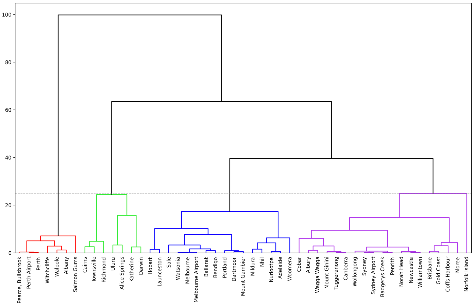
As you can see, we get quite different results when using the 'ward' linkage. The previous blue cluster has been split into two, and lonely Norfolk Island has been merged into the purple cluster.
HAC clustering - generating cluster labels
Since we have decided to have 4 clusters, let's run the scikit learn's HAC algorithm to generate cluster labels for both 'average' and 'ward' linkage methods.
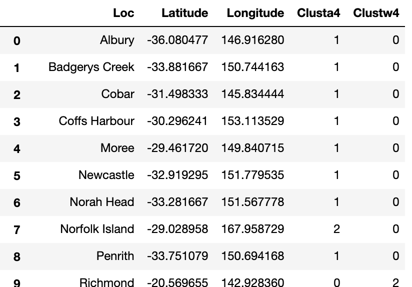
Finally, let's draw the results on a map.
Average linkage:
Ward linkage:
To plot clusters using 'ward,' we use the same Python code as above, except we change 'Clusta4' with 'Clustw4' in rows 5 and 8.
Conclusion
The nice thing about Hierarchical Agglomerative Clustering is that it gives you visibility on the proximity of all the data points through a dendrogram. This becomes even more important when you take your clustering to multi-dimensional space by using more than two attributes.
To summarize, I want to reiterate what I said in my K-Means article: clustering is rarely the end of your analysis; often, it is just the beginning. Hence, make sure to explore how you can use your newly created clusters to improve your understanding of the data and see how it can aid the development of other types of models.
Have fun using HAC in your projects, and feel free to let me know if you have any questions or suggestions!
Cheers! 👏 Saul Dobilas
If you liked this article, you might also enjoy a detailed explanation of the inner workings of other types of clustering algorithms:
K-Means Clustering - A Comprehensive Guide to Its Successful Use in Python
DBSCAN Clustering Algorithm - How to Build Powerful Density-Based Models
GMM: Gaussian Mixture Models - How to Successfully Use It to Cluster Your Data?