DBSCAN Clustering Algorithm - How to Build Powerful Density-Based Models
A detailed guide to using Density-Based Spatial Clustering of Applications with Noise
Machine Learning

Intro
If you want to be a successful Data Scientist, you need to understand the nuances of different Machine Learning algorithms.
This story is part of a series where I provide an in-depth look into how such algorithms work. This includes visualizations and real-life data examples with a complete Python code for you to use in your own Data Science projects.
Contents
What category of algorithms does DBSCAN belong to?
What are the different types of clustering algorithms?
How does the DBSCAN algorithm work?
Python example of using DBSCAN on real-life data.
What category of algorithms does DBSCAN belong to?
The total number of Machine Learning algorithms keeps growing over time, creating no shortage of ways to analyze your data. I have tried to collect and classify the most commonly used algorithms by the Data Science community. Make sure to explore the interactive sunburst chart below👇 by clicking on different categories to reveal more.
Note, in many cases, the same algorithm can be used to solve multiple types of problems. E.g., one can use Neural Networks for classification, regression, or as part of the reinforcement learning.
If you enjoy Data Science and Machine Learning, please subscribe to get an email whenever I publish a new story.
As indicated in the chart above, and as the name suggests (Density-Based Spatial Clustering of Applications with Noise), DBSCAN is a clustering algorithm, which falls under the Unsupervised branch of Machine Learning.
Typically one would use clustering to identify different groups (a.k.a. clusters) of customers, objects, or other types of data based on the similarity of chosen characteristics.
Types of clustering algorithms
Not all clustering algorithms are created equal. Different clustering algorithms implement different ideas on how to best cluster your data. There are 4 main categories:
Centroid-based - uses Euclidean distance to assign every point to the nearest cluster center. Example: K-Means
Connectivity-based - assumes that nearby objects (data points) are more related than far away objects. Example: Hierarchical Agglomerative Clustering (HAC).
Density-based - defines clusters as dense regions of space separated by low-density regions. Example: Density-Based Spatial Clustering of Applications with Noise (DBSCAN).
Distribution-based - assumes the existence of a specified number of distributions within the data. Each distribution with its own mean (μ) and variance (σ²) / covariance (Cov). Example: Gaussian Mixture Models (GMM).
How does the DBSCAN algorithm work?
Defining parameters
As mentioned above, density-based algorithms work by identifying dense regions in space (i.e., populated with many data points) separated by less dense regions. To enable the algorithm to find these dense regions, we first need to establish what we consider to be sufficiently dense. We do this by specifying two hyperparameters:
Epsilon (ϵ, sklearn: eps) - the radius of the area around the point defining the maximum distance between such point and any other points for one to be considered in the neighborhood of the other. In simple terms, it is the radius of the circle you can see in the below gif image.
Min points (MinPts, sklearn: min_samples) - the minimum number of points present in the neighborhood required to form a cluster.
Example
Let's look at the below example where eps=2.5 units, and MinPts=4. Note, iteration here refers to an algorithm iterating through each point and assigning it to one category (noise, core point, border point).
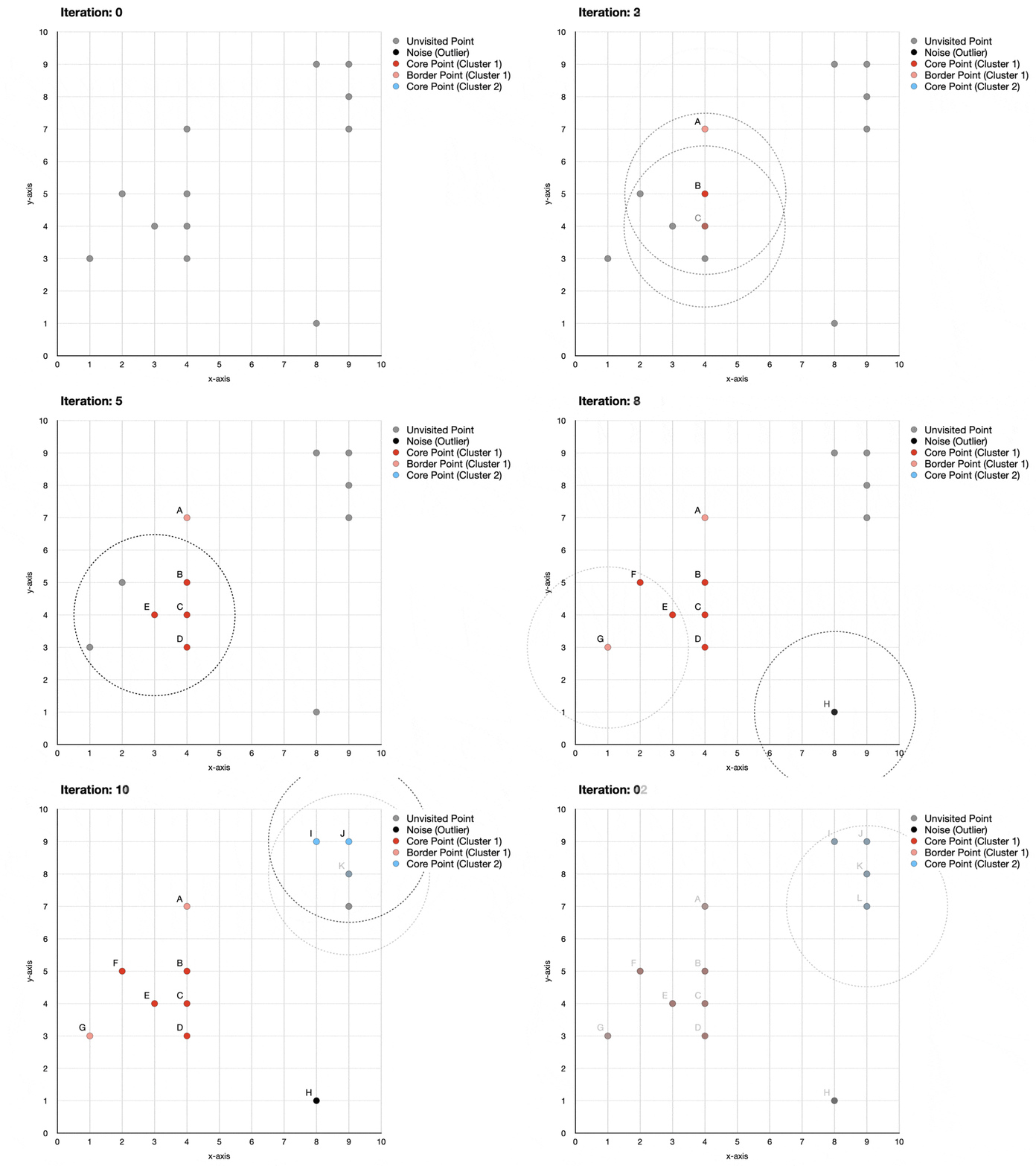
Iteration 0 - none of the points have been visited yet. Next, the algorithm will randomly pick a starting point taking us to iteration 1.
Iteration 1 - point A has only one other neighbor. Since 2 points (A+1 neighbor) is less than 4 (minimum required to form a cluster, as defined above), A is labeled as noise.
Iteration 2 - point B has 5 other points in its neighborhood. Since 6 points (B + 5 neighbors) is more than 4, the start of the first cluster is identified, with B becoming a core point. At the same time, previously considered to be noise, point A is relabeled as a border point since it sits within the neighborhood of core point B.
Iterations 3 to 6 - points C, D, E, F are labeled as core points and assigned to cluster 1.
Iteration 7 - point G is labeled as a border point because it is within the neighborhood of core points E and F but does not reach the minimum number of 4 points to be labeled as a core point.
Iteration 8 - point H is labeled as a noise (outlier) because there are no other points within its neighborhood.
Iterations 9 to 12 - a new cluster is identified and labeled, containing 4 core points (I, J, K, L).
Pros and cons of DBSCAN compared to other clustering methods
Pros: 1) Works well to identify arbitrarily shaped clusters; 2) can identify outliers which could potentially be the primary goal of the exercise.
Cons: It does not work well when there is varying density across the data since Epsilon and MinPts are fixed.

Python example of DBSCAN clustering
Now that we understand the DBSCAN algorithm let's create a clustering model in Python.
Setup
We will use the following data and libraries:
Scikit-learn library for 1) feature scaling (MinMaxScaler); 2) identifying optimal hyperparameters (Silhouette score); 3) performing DBSCAN clustering
Let's import all the libraries:
Next, we download and read in the data that we will use to build our DBSCAN clustering models. (source: https://www.kaggle.com/quantbruce/real-estate-price-prediction?select=Real+estate.csv)
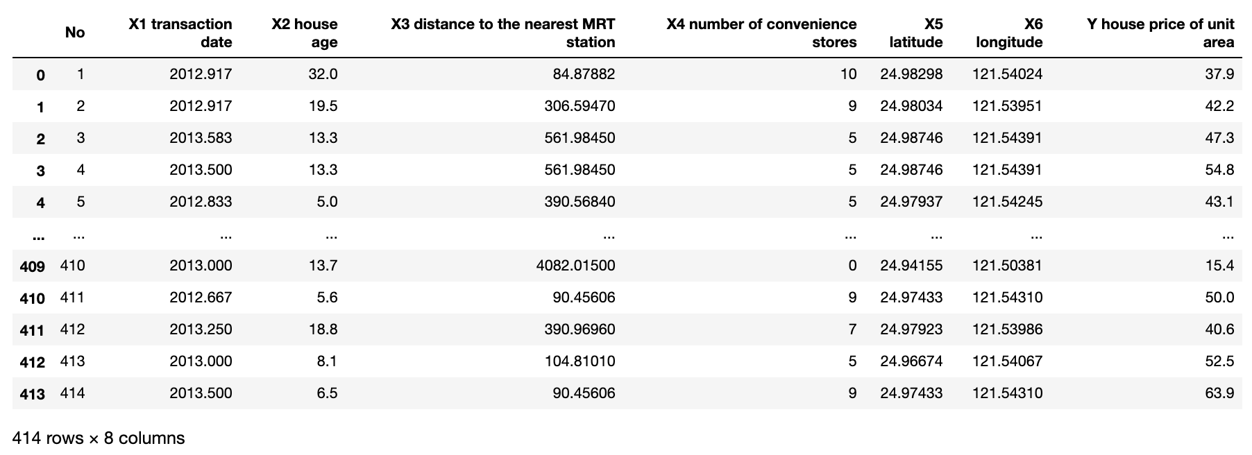
We will use the following 3 features to cluster the observations:
'X3 distance to the nearest MRT station'
'X2 house age'
'Y house price of unit area.'
Note, this data was meant to be used to predict house prices based on available features. That's why the field names start with X and Y, indicating what should be a feature and what should be a target. However, since we use it for a different purpose (i.e., clustering), we can ignore the naming convention.
Let's plot observations on a 3D graph.
Data preparation - feature scaling
When it comes to clustering, especially the density-based approach, it is crucial to prepare the data before putting it into the model. While you may want to perform multiple transformations, the most common one is scaling.
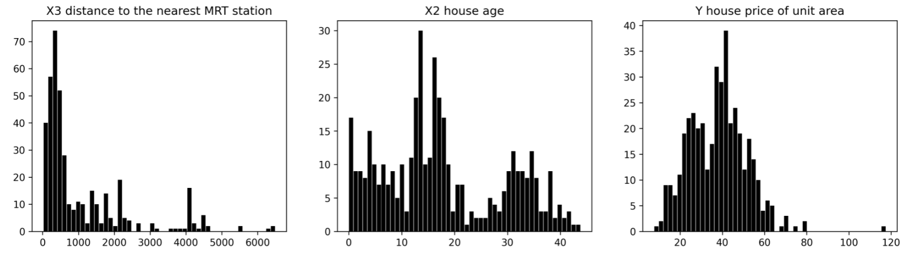
Scaling is done when your feature distributions have a very different range. E.g., in this example, the distance from the nearest MRT station ranges between 0 and 6,488, while house age ranges from 0 to 44. So they need to be scaled to fit them into the same range. Otherwise, it won't be easy to pick a value for epsilon, and one feature may end up being solely responsible for the outcome of clustering.
Let's plot distributions of our three features.
Now let's apply min-max scaling and plot it again.
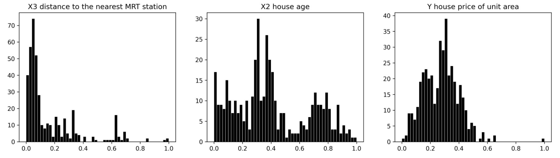
As you can see, min-max scaling did not affect the underlying distributions of the features. Instead, it scaled the range down, so all of them now fit in between 0 and 1.
In some scenarios, you may also want to apply transformations to the distribution. E.g., the distance to the nearest MRT looks similar to log distribution, meaning that most houses are located close to the station with few further away.
Therefore, if you were more interested in differentiating between all the houses close to the MRT and were less interested in the ones further away, then you could apply log transformation to spread them out.
DBSCAN clustering - selecting hyperparameter values
Now that we have our features prepped, let's decide on the values of epsilon and MinPts. For this, we will use the Silhouette score available in the sklearn library. Here is a direct quote from its documentation:
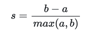
The Silhouette Coefficient is defined for each sample and is composed of two scores: a: The mean distance between a sample and all other points in the same class. b: The mean distance between a sample and all other points in the next nearest cluster.
The Silhouette Coefficient s for a single sample is then given as:
The Silhouette Coefficient for a set of samples is given as the mean of the Silhouette Coefficient for each sample.
Let's create multiple DBSCAN models using different combinations of epsilon and MinPts and plot Silhouette scores.
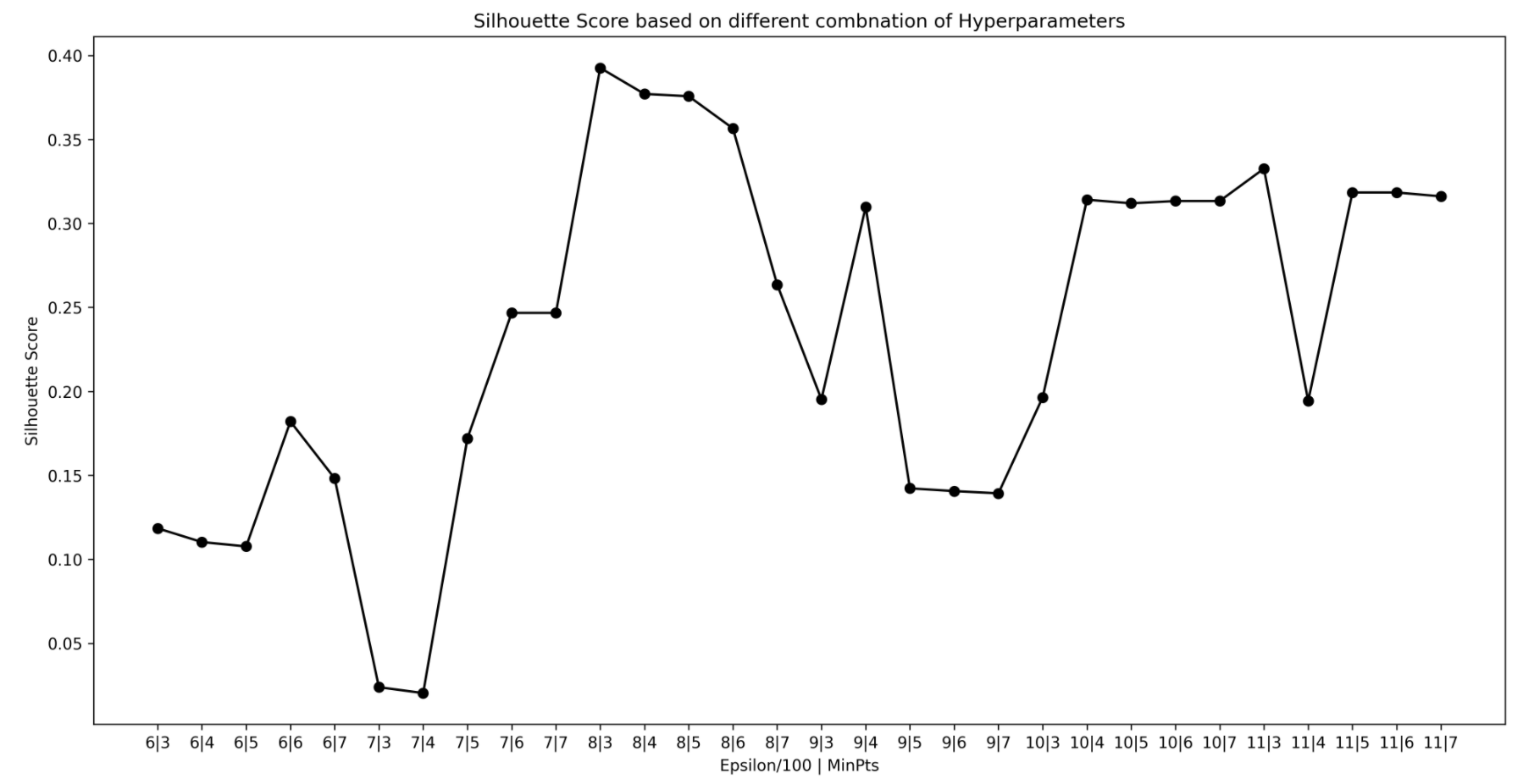
Looking at the above, we can see that eps=0.08 produce the highest scores. A few combinations ended up having very similar scores, indicating that the clustering output for those combinations would also be similar.
We will pick two different combinations to illustrate how the results vary on the choice of hyperparameters. We will use eps=0.08 and MinPts=3 for the first model and eps=0.06 and MinPts=6 for the second model.
DBSCAN clustering - running the algorithm
Let's build the models and print cluster labels:
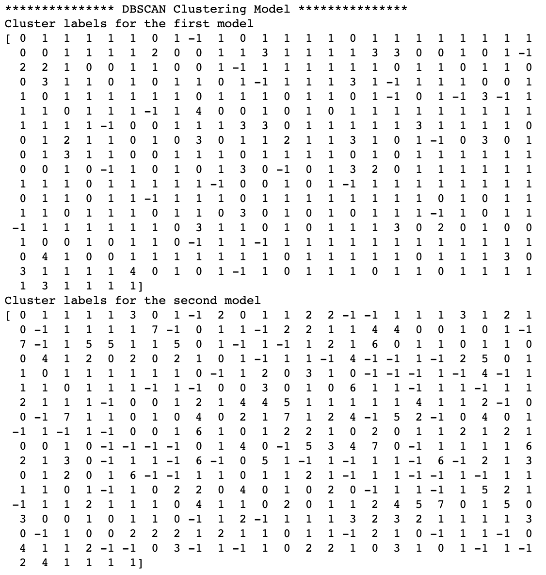
Note, -1 means the model defined the point as an outlier (noise).
You can immediately see that the first model (eps=0.08, MinPts=3) has fewer clusters, with clusters 0 and 1 being much larger than others. Meanwhile, the second model (eps=0.06, MinPts=6) produced many more clusters, which directly resulted from choosing smaller epsilon.
To make the results more visual, let's create the same 3D scatter plot using different colors for clusters.
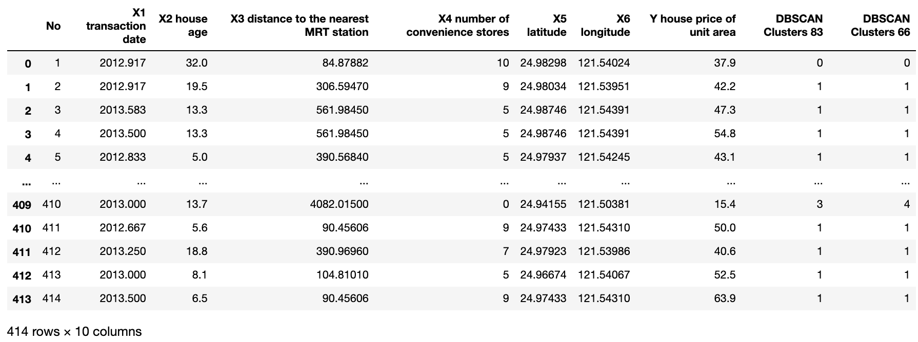
First, though let's merge cluster labels back to a data frame.
Plot a 3D chart for the first model (eps=0.08, MinPts=3).
Then we run the same code but replace ['DBSCAN Clusters 83'] with ['DBSCAN Clusters 66'].
As you can see, the second model has further split the two big clusters into a few smaller ones.
The formation of the two big clusters in the first model was driven by most houses being located close to the MRT station (see the distribution plot). While we mentioned that we could use log-transformation to spread out these observations, we took a different approach in the second model and reduced the epsilon value instead.
Conclusion
Density-based clustering is the approach you should consider when you have arbitrarily shaped clusters or when you are interested in finding outliers in your data.
Although, the major takeaway from this article should be that there isn't one right answer for clustering. Therefore, it is important to consider multiple preprocessing methods for your data and test a range of different hyperparameter values before generating the final clustering model.
I hope my Python code and detailed walkthrough of the algorithm has given you a good understanding of DBSCAN. In addition, I have listed a few links to alternative clustering algorithms if you wish to continue learning about this topic.
Cheers!👏 Saul Dobilas
GMM: Gaussian Mixture Models - How to Successfully Use It to Cluster Your Data?
HAC: Hierarchical Agglomerative Clustering. Is It Better Than K-Means?
K-Means Clustering - A Comprehensive Guide to Its Successful Use in Python