Random Forest Models: Why Are They Better Than Single Decision Trees?
A detailed explanation of how random forest machine learning algorithm works, what makes it superior to decision trees, and how you can...
Machine Learning
A detailed explanation of how random forest machine learning algorithm works, what makes it superior to decision trees, and how you can build them in Python
Intro
If you want to be a successful Data Scientist, you need to understand the nuances of different Machine Learning algorithms.
This story is part of a series where I provide an in-depth look at how such algorithms work. This includes simple examples, 3D visualizations, and complete Python code for you to use in your Data Science projects.
The story covers the following topics:
The category of algorithms Random Forest classification belongs to
An explanation of how Random Forest classification works and why it is better than a single decision tree
Python code examples and visualizations
What category of algorithms does it belong to?
Similar to some other algorithms, Random Forest can handle both classification and regression. While in this story, I focus on classification, the same logic largely applies to regression too.
A quick recap on the difference between classification and regression :
With classification, we attempt to predict a class label. In other words, it is used for problems where the output (target variable) takes a finite set of values, e.g., whether it will rain tomorrow or not. Corresponding algorithm:
[sklearn.ensemble.RandomForestClassifier](https://scikit-learn.org/stable/modules/generated/sklearn.tree.DecisionTreeClassifier.html#sklearn-tree-decisiontreeclassifier)Meanwhile, regression is used to predict a numerical label. This means your output can take an infinite set of values, e.g., a house price. Corresponding algorithm:
[sklearn.ensemble.RandomForestRegressor](https://scikit-learn.org/stable/modules/generated/sklearn.ensemble.RandomForestRegressor.html)
Both cases fall under the supervised branch of machine learning algorithms. The below graph is interactive, so make sure to click on different categories to enlarge and reveal more👇 .
If you enjoy Data Science and Machine Learning, please subscribe to get an email whenever I publish a new story.
How does the Random Forest classification algorithm work?
Under the hood, the random forest is essentially a CART algorithm (Classification and Regression Trees), except it creates an ensemble of many trees instead of just one. This provides several advantages such as:
Improved performance (the wisdom of crowds)
Improved robustness (less likely to overfit since it relies on many random trees)
If you are not familiar with CART, you can find everything about it in my previous story:
CART: Classification and Regression Trees for Clean but Powerful Models
Wisdom of crowds - what is it and why is it good?
Random Forest algorithm uses majority agreement prediction for the class label, which means that each tree predicts whether the observation belongs to 'Class 0' or 'Class 1'. If 55 trees out of a hundred predicted 'Class 1' and 45 predicted 'Class 0', then the final model prediction would be 'Class 1'.
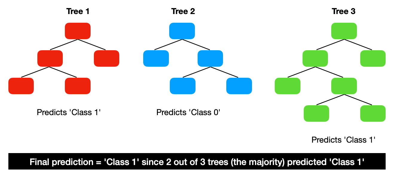
The majority prediction from multiple trees is better than an individual tree prediction because the trees protect each other from their individual errors. This is, however, dependant on the trees being relatively uncorrelated with each other.
The process of building multiple trees
The question is - how do we build many trees from the same data pool while keeping them relatively uncorrelated? There are two parts to it:
Bootstrap aggregation (random sampling with replacement)
Feature randomness
Bootstrap aggregation
Decision trees are so-called high-variance estimators, which means that small changes to the sample data can greatly impact the tree structure and its prediction.
Ideally, you want to turn it into a low-variance estimator by creating many trees and using them in aggregation to make the prediction.
Bootstrapping is a technique where instead of taking the whole training data to build one tree, you use sampling with replacement to create many samples of the same size. Then you can use these samples to build separate trees. For example:
In this case, you randomly pick one number from the whole sample and record what you have picked. Then you repeat the action until you have recorded 10 observations.
An equivalent would be randomly picking a ball from a bucket of red and blue balls, recording its color, and then returning it to the bucket before repeating the same action.
This method produces many samples with the same observations but different distributions. In the end, the aggregation of these trees leads to a reduction in the variance of your model prediction, turning it into a low-variance estimator.
Feature randomness
The second part in reducing the correlation between the trees comes from using a random selection of features when looking for the best split for each node.
For example:
This process allows the creation of less correlated trees and, combined with bootstrap aggregation, produces a Random Forest.

Python examples of Random Forest classification models
Leaving theory behind, let us build a Random Forest model in Python.
Setup
We will use the following data and libraries:
Scikit-learn library for splitting the data into train-test samples, building Random Forest models, and model evaluation
Plotly for data visualizations
Graphviz library to plot decision tree graphs
Let's import all the libraries:
Then we get the Australian weather data from Kaggle, which you can download following this link: https://www.kaggle.com/jsphyg/weather-dataset-rattle-package.
We ingest the data and derive a few new variables for usage in the models.
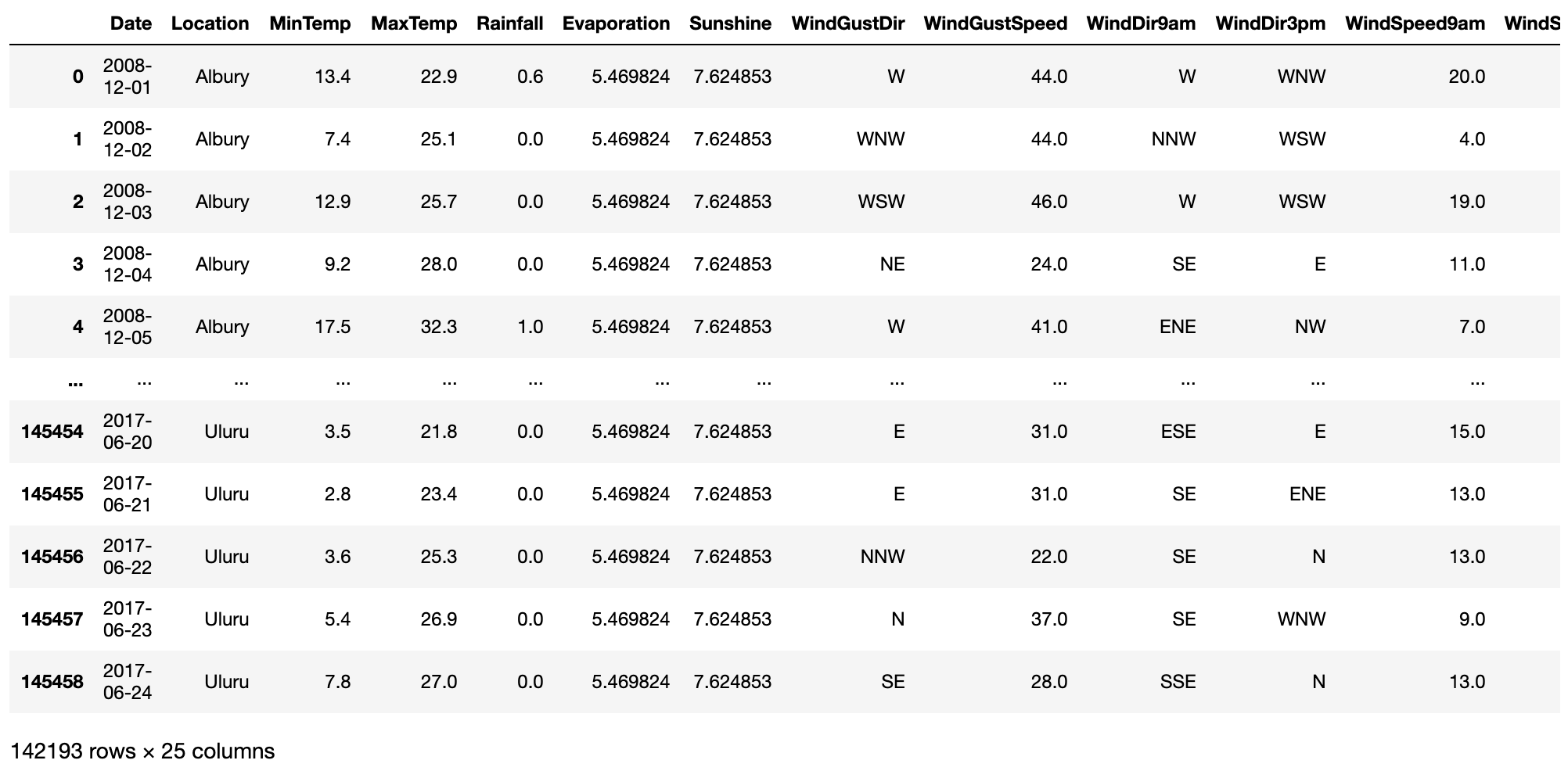
Next, let's build a model by following these steps:
Step 1 - select model features (independent variables) and model target (dependent variable)
Step 2 - split data into train and test samples
Step 3 - set model parameters and train (fit) the model
Step 4 - predict class labels on train and test data using our model
Step 5 - generate model summary statistics
The above code generates the following output that summarizes the model performance.
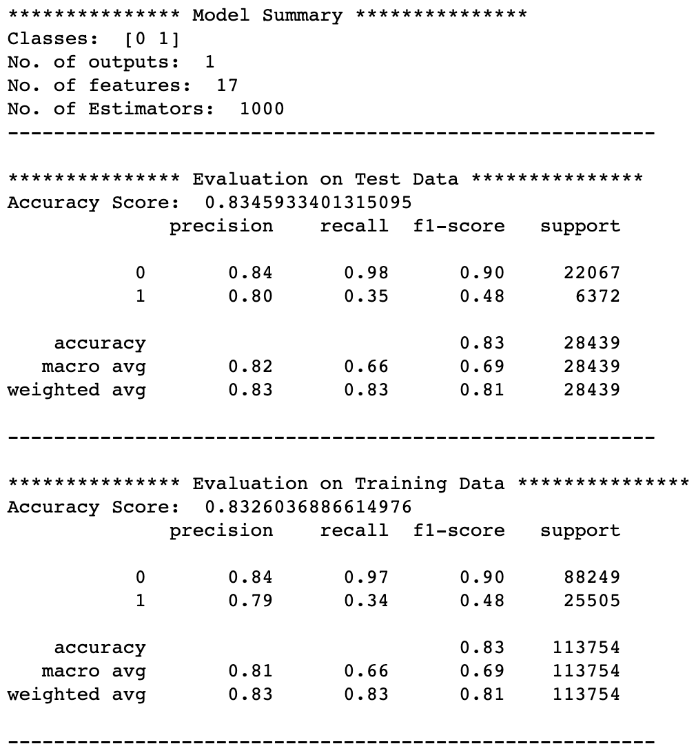
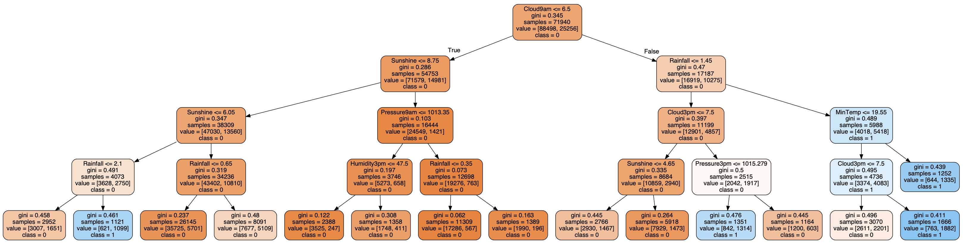
As we can see, the model generalized quite well with similar performance on test data when compared to training data. The number of estimators was 1000, which means that our Random Forest consists of 1000 individual trees. Here is what a tree 552 looks like. If you wish, you can generate tree diagrams for each one of them by changing the index.
Bonus code
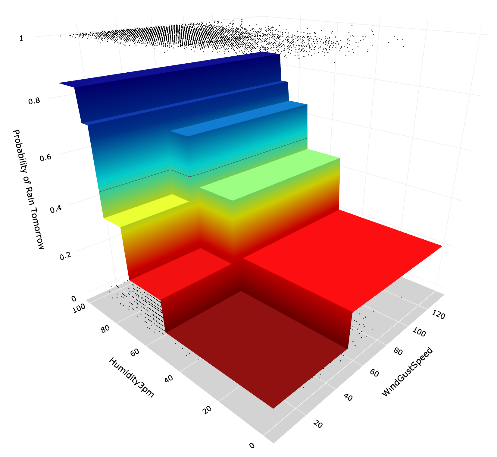
While we cannot easily visualize all model predictions using 17 features, we can do it when we build a random forest with just 2 features. For this, we first need to build another model using the code above, remembering to select only 2 features:
After building a model, we use the following code to create a 3D visualization with Plotly:
The above generates the following graph.
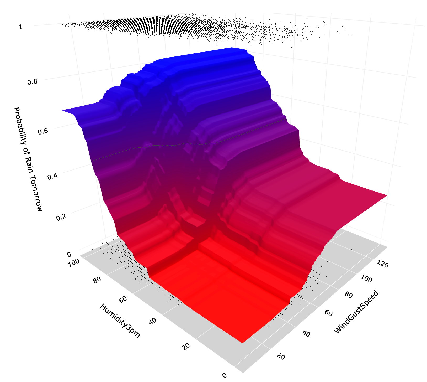
From the above visualization, we can clearly see that chances of rain tomorrow increase as the humidity at 3 pm and wind gust speed increases. Also, while not completely smooth, the decision surface has fewer big step changes compared to using just one decision tree (see graph below).
Conclusion
Random Forest is amongst the best performing Machine Learning algorithms, which has seen wide adoption. While it is a bit harder to interpret than a single Decision Tree model, it brings many advantages, such as improved performance and better generalization.
Thanks for reading, and feel free to use the above code and materials in your own Data Science projects.
Cheers! 👏 Saul Dobilas
Also, you may be interested to see how Random Forest compares to AdaBoost:
AdaBoost Machine Learning Algorithm: How to Improve Performance of Hard to Predict Cases
Other Boosting Algorithms:
Gradient Boosted Trees for Classification - One of the Best Machine Learning Algorithms
XGBoost: Extreme Gradient Boosting - How to Improve on Regular Gradient Boosting?