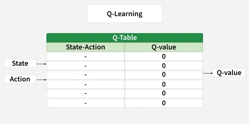
Deep Q-Learning in Reinforcement Learning

Deep Q-Learning (DQL) is a Deep Reinforcement Learning algorithm that combines the principles of Q-Learning with deep neural networks to solve complex decision-making problems. Instead of storing Q-values in a lookup table, it uses a neural network to approximate the Q-value function.

• Q-Value: Represents the expected cumulative reward that an agent can obtain by taking a particular action in a given state and following the optimal policy thereafter.
• Deep Neural Network: Learns complex patterns from data and approximates the Q-value function instead of storing values in a traditional Q-table.
• High-Dimensional State Space: Refers to environments with a very large number of possible states, such as images, videos, or sensor readings, where maintaining a Q-table becomes impractical.
• Decision-Making: Enables an agent to learn the best sequence of actions through trial-and-error interactions with the environment to maximize long-term rewards.

Mathematical Formulation

Deep Q-Learning approximates the optimal Q-value function using a deep neural network:

Q(s,a;\theta)\approx Q^*(s,a)

Where:

• Q(s,a;\theta) = Q-value predicted by the neural network
• Q^*(s,a) = Optimal Q-value
• \theta = Neural network parameters

Architecture of Deep Q-Networks

A DQN consists of the following components:

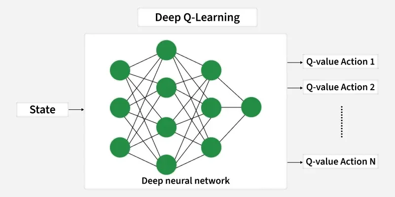
1. Neural Network

• The network approximates the Q-value function Q(s,a;θ) where \theta represents the trainable parameters.
• For example in Atari games the input might be raw pixels from the game screen and the output is a vector of Q-values corresponding to each possible action.

2. Experience Replay

• To stabilize training, DQNs store past experiences (s,a,r,s′) in a replay buffer.
• During training, mini-batches of experiences are sampled randomly from the buffer, breaking the correlation between consecutive experiences and improving generalization.

3. Target Network

• A separate target network with parameters \theta^{-} is used to compute the target Q-values during updates. The target network is periodically updated with the weights of the main network to ensure stability.

4. Loss Function

• The loss function measures the difference between the predicted Q-values and the target Q-values:

L(\theta)= E[(r+\gamma \max_{a'}Q(s', a'; \theta^{-}) - Q(s,a; \theta))^2]

Training Process

The training process of a DQN involves the following steps:

1. Initialization:

• Initialize the replay buffer, main network (\theta) and target network (\theta^{-}).
• Set hyperparameters such as learning rate (\alpha), discount factor (\gamma) and exploration rate (\epsilon).

2. Exploration vs. Exploitation: Use an \epsilon-greedy policy to balance exploration and exploitation:

• With probability \epsilon, select a random action to explore.
• Otherwise, choose the action with the highest Q-value according to the current network.

3. Experience Collection: Interact with the environment, collect experiences (s,a,r,s′) and store them in the replay buffer.

4. Training Updates:

• Sample a mini-batch of experiences from the replay buffer.
• Compute the target Q-values using the target network.
• Update the main network by minimizing the loss function using gradient descent.

5. Target Network Update: Periodically copy the weights of the main network to the target network to ensure stability.

6. Decay Exploration Rate: Gradually decrease \epsilon over time to shift from exploration to exploitation.

Implementing Deep Q-Network for the CartPole Environment

In this implementation, we train a Deep Q-Network (DQN) agent to balance a pole on a moving cart.

Step 1: Install the Required Libraries

• Gymnasium provides reinforcement learning environments such as CartPole.
• TensorFlow is used to build and train the Deep Q-Network.
• NumPy performs numerical operations.

!pip install gymnasium tensorflow numpy

Step 2: Import the Required Libraries

• Imports Gymnasium to create the environment.
• Imports NumPy for numerical computations.
• Imports TensorFlow to build the neural network.

import gymnasium as gym
import numpy as np
import tensorflow as tf
from tensorflow.keras.models import Sequential
from tensorflow.keras.layers import Dense

Step 3: Create the CartPole Environment

• Creates the CartPole environment.
• Retrieves the number of input features (states).
• Retrieves the total number of possible actions.

env = gym.make("CartPole-v1")

state_size = int(env.observation_space.shape[0])
action_size = int(env.action_space.n)

print("State Size:", state_size)
print("Action Size:", action_size)

Output:

State Size: 4

Action Size: 2

Step 4: Build the Deep Q-Network

• Creates a simple neural network with one hidden layer.
• Uses ReLU activation for learning complex patterns.
• Uses a linear output layer to predict Q-values.
• Compiles the model using the Adam optimizer and MSE loss.

model = Sequential([
    Dense(24, activation="relu", input_shape=(state_size,)),
    Dense(action_size, activation="linear")
])

model.compile(optimizer="adam", loss="mse")

Step 5: Define the Hyperparameters

• Gamma determines the importance of future rewards.
• Epsilon controls exploration during training.
• Epsilon Decay gradually reduces random actions.
• Episodes specify how many times the agent interacts with the environment.

gamma = 0.95
epsilon = 1.0
epsilon_decay = 0.99
epsilon_min = 0.01
episodes = 50

Step 6: Train the DQN Agent

• Resets the environment at the beginning of each episode.
• Selects either a random action or the best predicted action using the ε-greedy strategy.
• Executes the action and receives the next state and reward.
• Updates the Q-value using the Bellman equation.

for episode in range(episodes):

    state, _ = env.reset()
    state = state.reshape(1, state_size)

    done = False

    while not done:

        if np.random.rand() < epsilon:
            action = env.action_space.sample()
        else:
            action = np.argmax(model.predict(state, verbose=0))

        next_state, reward, terminated, truncated, _ = env.step(action)
        done = terminated or truncated
        next_state = next_state.reshape(1, state_size)

        target = reward
        if not done:
            target += gamma * np.max(model.predict(next_state, verbose=0))

        q_values = model.predict(state, verbose=0)
        q_values[0][action] = target

        model.fit(state, q_values, epochs=1, verbose=0)
        state = next_state

    epsilon = max(epsilon_min, epsilon * epsilon_decay)

    print(f"Episode {episode+1} completed")

Output:

Episode 1 completed
Episode 2 completed
...
Episode 50 completed

Step 7: Test the Trained Agent

• Uses the trained model to choose the best action.
• Runs the agent until the episode ends.
• Calculates the total reward obtained.
• Displays the final performance of the trained agent.

state, _ = env.reset()
state = state.reshape(1, state_size)

done = False
total_reward = 0

while not done:

    action = np.argmax(model.predict(state, verbose=0))

    next_state, reward, terminated, truncated, _ = env.step(action)

    total_reward += reward
    state = next_state.reshape(1, state_size)
    done = terminated or truncated

print("Total Reward:", total_reward)

Output:

Total Reward: 9.0

You can download the complete code from here.

Applications

• Atari Games: It can learn to play old video games very well even better than humans by looking at the screen pixels.
• Robotics: It helps robots to learn how to pick objects, move around and do tasks with their hands.
• Self-Driving Cars: It helps cars to make decisions like changing lanes and avoiding obstacles safely.
• Finance: It is used to find the best ways to trade stocks, manage money and reduce risks.
• Healthcare: It helps with planning treatments, discovering new medicines and personalizing care for patients.

Advantages

• Can handle high-dimensional state spaces using deep neural networks instead of Q-tables.
• Learns directly from raw inputs such as images, videos, and sensor data without manual feature engineering.
• Experience Replay improves sample efficiency by reusing past experiences during training.
• Target Networks stabilize learning by reducing oscillations in Q-value updates.
• Can solve complex sequential decision-making problems in robotics, gaming, and autonomous systems.
• Eliminates the need to store enormous Q-tables for large environments.

Limitations

• Requires significant computational resources and GPU acceleration for efficient training.
• Needs a large number of interactions with the environment before learning an effective policy.
• Primarily designed for discrete action spaces and is not well suited for continuous control tasks.
• Training performance is sensitive to hyperparameter selection, such as learning rate and exploration rate.
• May exhibit unstable learning if replay buffers or target networks are not properly configured.

Related Articles

• Reinforcement Learning
• Double Deep Q-Network (Double DQN)