
A uniform distribution is a type of probability distribution in which every outcome in a given range is equally likely to occur. That means there is no bias; no outcome is more likely than another within the specified set.
- It has two parameters, a and b: a = minimum and b = maximum. The distribution is written as U (a, b).
- For example: Rolling a fair six-sided die: Each number (1, 2, 3, 4, 5, or 6) has an equal chance of being rolled, with a probability of
\frac{1}{6} for each outcome.
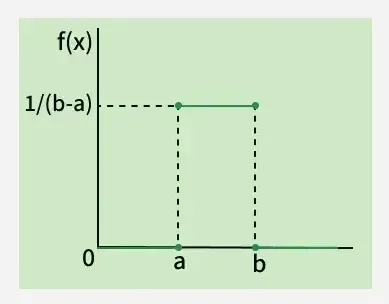
The graph represents a continuous uniform distribution on the interval [a, b].
- The graph is a Uniform Distribution on the interval [a, b].
- The probability density f(x)is constant between a and b.
- The height of the graph is
\frac{1}{b-a} , meaning the total area equals 1.- The graph is a rectangle between a and b, illustrating that all values in that range have equal likelihood.
There are two main types of uniform distribution:
1. Discrete Uniform Distribution
Discrete uniform distribution is a probability distribution that describes the likelihood of outcomes when each outcome in a finite set is equally likely. It's characterized by a constant probability mass function (PMF) over a finite range of values.
Its properties and applications extend across various disciplines, making it a versatile tool in data analysis and decision-making processes.
P(X=x_i) = \frac{1}{n}, for \: i=1,2,…,n
Example: Rolling fair dice or flipping fair coins, where each outcome has an equal probability.
Estimation of Maximum
In statistics, the estimation of the maximum refers to methods used to estimate the largest value or the maximum observation in a dataset. Techniques such as order statistics and maximum likelihood estimation are commonly employed for this purpose.
Random Permutation
A random permutation is a random arrangement of a set of items or elements. It's often used in various fields such as cryptography, statistics, and computer science. Generating random permutations is essential in algorithms, simulations, and experimental designs.
Graph of Discrete Uniform Distribution
Rolling a Fair Die
- When rolling a fair six-sided die, each face (1, 2, 3, 4, 5, 6) has an equal probability of 1/6 of landing face up.
- This is a classic example of a discrete uniform distribution.
Graph: Probability Mass Function (PMF) of Rolling a Fair Die
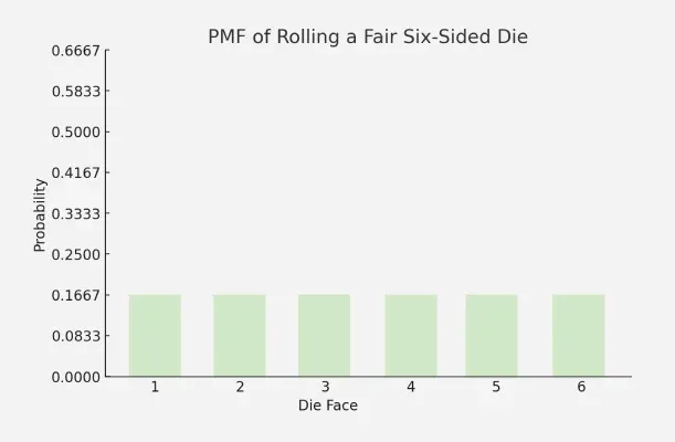
The graph for this example will show each possible outcome (1 through 6) on the x-axis and the probability (1/6) on the y-axis.
Properties
- Each outcome in the sample space has an equal probability of occurrence.
- The probability mass function (PMF) is constant over the range of possible outcomes.
- The mean of a discrete uniform distribution is the average of the minimum and maximum values.
- The variance of a discrete uniform distribution is
[\frac{(n^2 - 1)}{12}] , where n is the number of possible outcomes.
Applications
- Modeling scenarios where there is no preference or bias towards any particular outcome.
- Sampling without replacement, such as selecting random samples from a finite population.
- Generating random numbers for simulations, Monte Carlo methods, and randomized algorithms.
- Creating random permutations for shuffling decks of cards, designing experiments, and cryptographic applications.
2. Continuous Uniform Distributions
Continuous uniform distributions, also known as rectangular distributions, are probability distributions where the probability density function (PDF) is constant within a certain interval and zero elsewhere. This means that all outcomes within the interval are equally likely.
Continuous uniform distributions provide a simple yet powerful framework for understanding and modeling randomness within defined intervals, making them essential tools in probability theory and applied statistics.
Example: Generating a random number between 0 and 1.
Note: The density is constant and non-zero over an interval. The probability at a particular point is always zero.
P(a ≤ X ≤ b) = 1 (entire interval).
P(X = x) = 0 for any exact value of x.
Probability Density Function (PDF)
The probability density function (PDF) of a continuous uniform distribution defines the probability of a random variable falling within a particular interval. For a continuous uniform distribution over the interval [a, b], the PDF is given by:
f(x) =
\frac{1}{(b - a)} for a ≤ x ≤ b and f(x) = 0 otherwise.
The height of the PDF is constant between a and b.
- The total area under the curve (which represents the total probability) is 1.
- Every value within the interval is equally likely.
Cumulative Distribution Function (CDF)
The cumulative distribution function (CDF) of a continuous uniform distribution gives the probability that a random variable is less than or equal to a certain value. For the continuous uniform distribution over [a, b], the CDF is defined as:
F(x) = (x - a) / (b - a) for a ≤ x ≤ b and F(x) = 0 for x < a, F(x) = 1 for x > b.
- For values less than a: the probability is 0.
- For values greater than b, the probability is 1.
- For values within the interval [a, b]: probability increases linearly from 0 to 1.
This function is a rising straight line between a and b, showing how probability accumulates across the interval.
Generating Functions
Generating functions provide a way to represent sequences of numbers as power series. In probability theory, generating functions are often used to manipulate sequences of random variables. They can simplify calculations and help derive important properties of random variables and distributions.
Standard Uniform Distribution
The standard uniform distribution is a special case of the continuous uniform distribution where the interval is [0, 1]. It is widely used in simulations, random number generation, and various statistical applications.
Graph of Continuous Uniform Distribution
Random Number Generation: Suppose a random number generator is programmed to produce a real number between 0 and 1, with each number in this range being equally likely. This is an example of a continuous uniform distribution.
Graph: Probability Density Function (PDF) of Random Number Generation
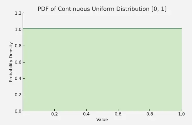
The graph will show the range [0, 1] on the x-axis, with a constant probability density of 1 across this interval.
Properties
- Equal probability density within the interval.
- Cumulative distribution function increases linearly within the interval.
- The mean of a continuous uniform distribution is the midpoint of the interval.
- The variance of a continuous uniform distribution is
\frac{[(b - a)^2]}{12} .
Applications
- Modeling uncertainty in various fields such as engineering, finance, and physics.
- Random number generation for simulations and games.
- Used in statistical quality control to model uniformity in manufacturing processes.
- In cryptography generate keys and create random permutations.
- As a baseline distribution for comparison with other distributions in statistical analysis.
Formulas
A random variable X is said to be uniformly distributed over the interval -∞ < a < b < ∞. Formulae for uniform distribution:
| Probability density function(pdf) | f(x) = |
|---|---|
| Mean(μ) | = |
| Variance (σ2 ) | = μ2' - μ2 = = |
| Standard Deviation (σ) | |
| Cumulative Distribution function (CDF) | = |
| Median | = |
| For the conditional probability = P( c < x < d ) | = (d - c ) × f(x) |
➢Practice: Solved Examples
