Graphing a Function in Python Using Plotnine Library

Plotnine library is a Python data visualization library based on the Grammar of Graphics, inspired by R's ggplot2. It provides a simple and expressive way to create high-quality visualizations by combining data, aesthetics, and graphical elements.

Installation

Before creating plots, install Plotnine using the following command:

pip install plotnine

After installation, you can import the library and use it to create a wide variety of plots, including function graphs, scatter plots, bar charts, histograms, and more.

Plotting a Simple Function

Let’s begin by graphing a simple linear function f(x) = 2x+1. We’ll first define the function and generate data points, then use Plotnine to visualize the function.

To plot the function, we first need to generate a set of values for the independent variable x and compute the corresponding y values using the function.

import pandas as pd
import numpy as np

x = np.linspace(-10, 10, 100)
y = 2 * x + 1
df = pd.DataFrame({'x': x, 'y': y})

Now, we’ll create a basic line plot using the geom_line() function from Plotnine, which is used to visualize continuous data.

from plotnine import ggplot, aes, geom_line
plot = (ggplot(df, aes(x='x', y='y')) + geom_line())
print(plot)

Output

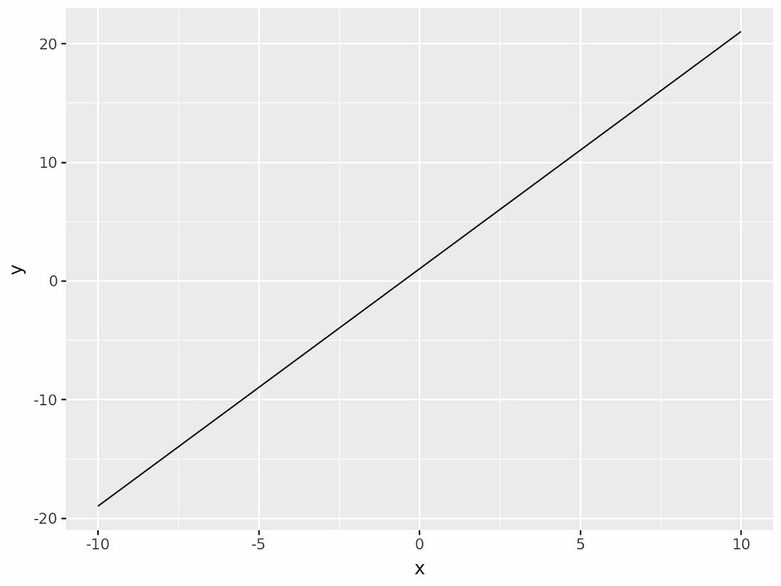
This code will create a simple line graph showing the linear relationship between x and y.

Customizing the Plot

The power of Plotnine lies in its ability to customize plots extensively. In this section, we’ll explore how to modify the appearance of our graph, from colors to titles and axis labels.

1. Adding Titles and Labels

It’s essential to make your plot informative by adding titles and axis labels.

from plotnine import ggtitle, xlab, ylab

plot = ( ggplot(df, aes(x='x', y='y')) +
         geom_line(color="blue") +
         ggtitle('Graph of Linear Function: y = 2x + 1') +
         xlab('x values') +
         ylab('y values') )
print(plot)

Output

2. Modifying Line Appearance

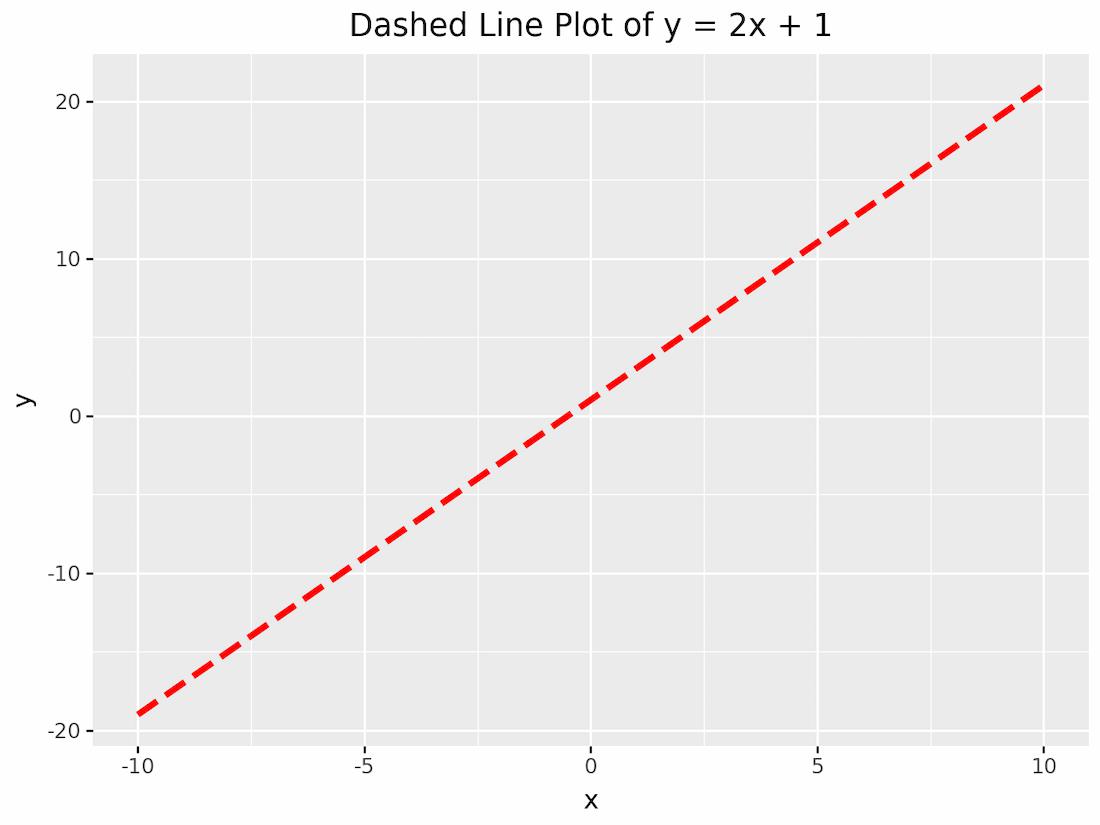
You can change the appearance of the line by modifying parameters such as color, linetype, and size.

plot = (ggplot(df, aes(x='x', y='y')) +
        geom_line(color="red", linetype="dashed", size=1.5) +
        ggtitle('Dashed Line Plot of y = 2x + 1'))

print(plot)

Output

Plotting Non-linear Functions

In addition to linear functions, Plotnine can be used to visualize non-linear functions such as quadratic, cubic, and trigonometric functions.

1. Quadratic Function

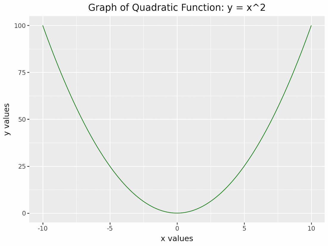
Let’s plot a quadratic function f(x)=x^2

y = x ** 2
df = pd.DataFrame({'x': x, 'y': y})

plot = (ggplot(df, aes(x='x', y='y')) +
        geom_line(color="green") +
        ggtitle('Graph of Quadratic Function: y = x^2') +
        xlab('x values') +
        ylab('y values'))

print(plot)

Output

2. Cubic Function

A cubic function like f(x)=x^3 can also be plotted similarly:

y = x ** 3
df = pd.DataFrame({'x': x, 'y': y})

plot = (ggplot(df, aes(x='x', y='y')) +
        geom_line(color="purple") +
        ggtitle('Graph of Cubic Function: y = x^3'))

print(plot)

Output

3. Trigonometric Functions

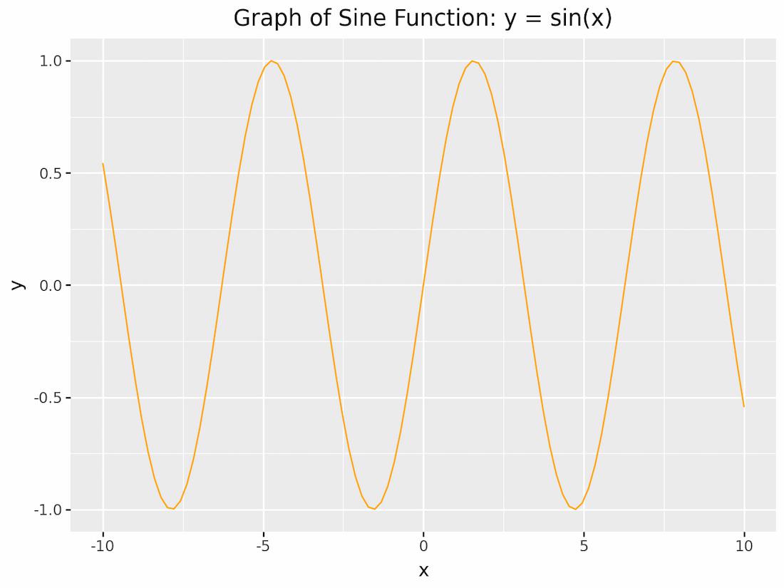
Plotting trigonometric functions such as sine or cosine is just as easy. Let’s graph f(x)=sin(x).

y = np.sin(x)
df = pd.DataFrame({'x': x, 'y': y})

plot = (ggplot(df, aes(x='x', y='y')) +
        geom_line(color="orange") +
        ggtitle('Graph of Sine Function: y = sin(x)'))

print(plot)

Output

Overlaying Multiple Functions

You can also plot multiple functions on the same graph by adding multiple geom_line() layers. Let’s plot both the quadratic and sine functions on the same graph for comparison.

y1 = x ** 2
y2 = np.sin(x)
df = pd.DataFrame({'x': x, 'y1': y1, 'y2': y2})

plot = (ggplot(df) +
        geom_line(aes(x='x', y='y1'), color="blue") +
        geom_line(aes(x='x', y='y2'), color="red") +
        ggtitle('Graph of y = x^2 and y = sin(x)') +
        xlab('x values') +
        ylab('y values'))

print(plot)

Output

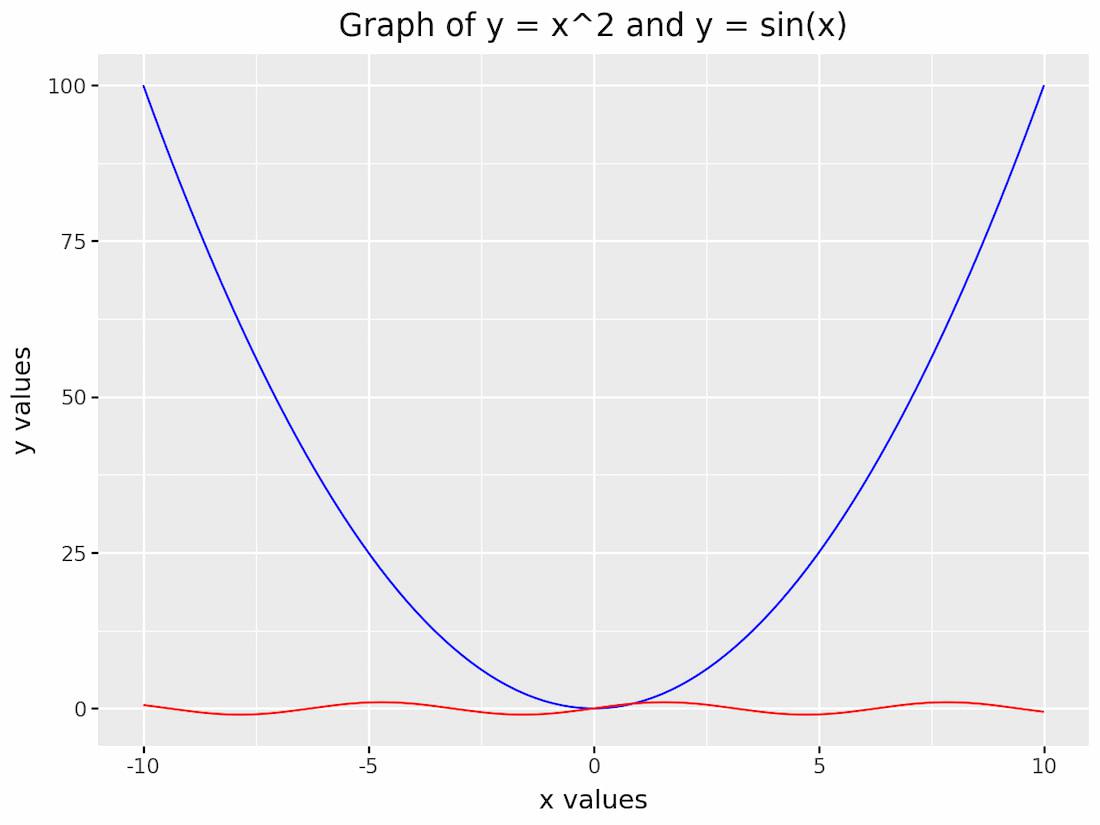
This code will create a plot that overlays the quadratic and sine functions, with different colors to distinguish between them.

Facetting Plots by Function Type

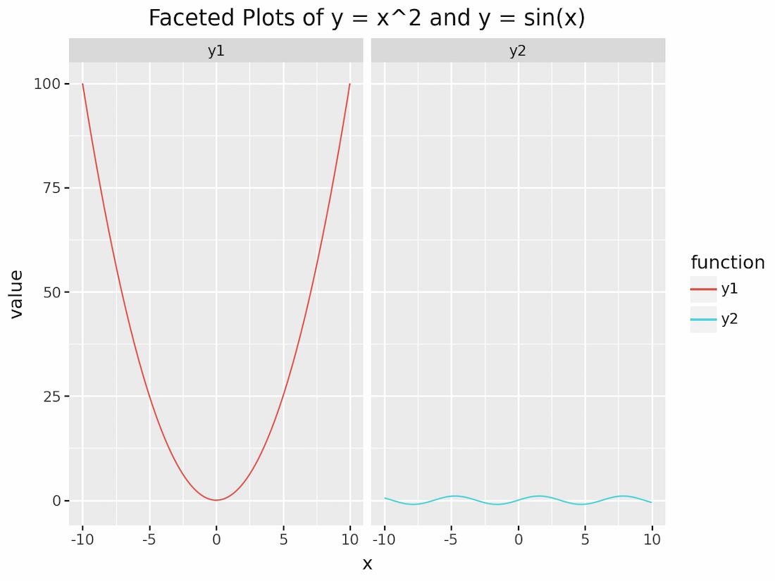
Another powerful feature of Plotnine is its ability to facet data. This means breaking a plot into multiple subplots based on the values of a variable. Faceting is particularly useful when you want to compare multiple functions or datasets side by side.

Let’s create two subplots for the quadratic and sine functions using facet_wrap().

from plotnine import ggplot, aes, geom_line, facet_wrap, ggtitle
import pandas as pd
import numpy as np

x = np.linspace(-10, 10, 100)
y1 = x ** 2
y2 = np.sin(x)
df = pd.DataFrame({'x': x, 'y1': y1, 'y2': y2})
df_melted = pd.melt(df, id_vars=['x'], value_vars=['y1', 'y2'], var_name='function')

plot = (ggplot(df_melted, aes(x='x', y='value', color='function')) +
        geom_line() +
        facet_wrap('~function') +
        ggtitle('Faceted Plots of y = x^2 and y = sin(x)'))

print(plot)

Output